SoK: Privacy-Preserving Data Synthesis
Back to home page
Additional Experimental Results
Table of Contents
Runtime of Different Approaches
We evaluate six DL-based approaches on two datasets (MNIST and Fashion-MNIST), under five scenarios (non-private, two standard, and two challenging).
We report the runtime of different approaches. For each scenario, we report the runtime for the run using the best hyper-parameters (reported in Evaluation Setups).
The results are presented in Table 1. The numbers are in seconds.
To summarize, DP-MERF is the most efficient algorithm and finishes within a minute. This can be attributed to its simple optimization procedure. DPGEN is most time-consuming, due to the sample efficiency issues of diffusion models.
Table 1: Runtime comparisons between different approaches. The numbers are in seconds.
Table 1-a: MNIST.
| non-private | $\varepsilon=10$ | $\varepsilon=1$ | $\varepsilon=0.2$ | half | |
|---|---|---|---|---|---|
| DPGAN | 1090.2 | 698.8 | 927.3 | 45.9 | 399.7 |
| DP-CGAN | 859.0 | 881.6 | 525.3 | 157.1 | 832.7 |
| GS-WGAN | 8107.9 | 6728.5 | 1344.3 | 65.0 | 8574.1 |
| DP-MERF | 53.7 | 35.9 | 39.0 | 36.5 | 41.5 |
| DP-Sinkhorn | 634.0 | 29626.0 | 13497.0 | 15087.0 | 42280.0 |
| DPGEN | 194106.0 | 149766.0 | 213196.0 | 124279.0 | 188399.0 |
Table 1-b: Fashion-MNIST.
| non-private | $\varepsilon=10$ | $\varepsilon=1$ | $\varepsilon=0.2$ | half | |
|---|---|---|---|---|---|
| DPGAN | 1059.7 | 934.0 | 921.3 | 39.3 | 371.3 |
| DP-CGAN | 966.6 | 859.1 | 1064.1 | 145.4 | 814.7 |
| GS-WGAN | 9671.6 | 6590.5 | 2466.7 | 170.0 | 8215.8 |
| DP-MERF | 53.6 | 28.2 | 34.2 | 41.6 | 32.8 |
| DP-Sinkhorn | 649.0 | 14668.0 | 24140.0 | 16641.0 | 36090.0 |
| DPGEN | 193837.0 | 146750.0 | 105233.0 | 126115.0 | 188053.0 |
Visualization of Synthesized Images
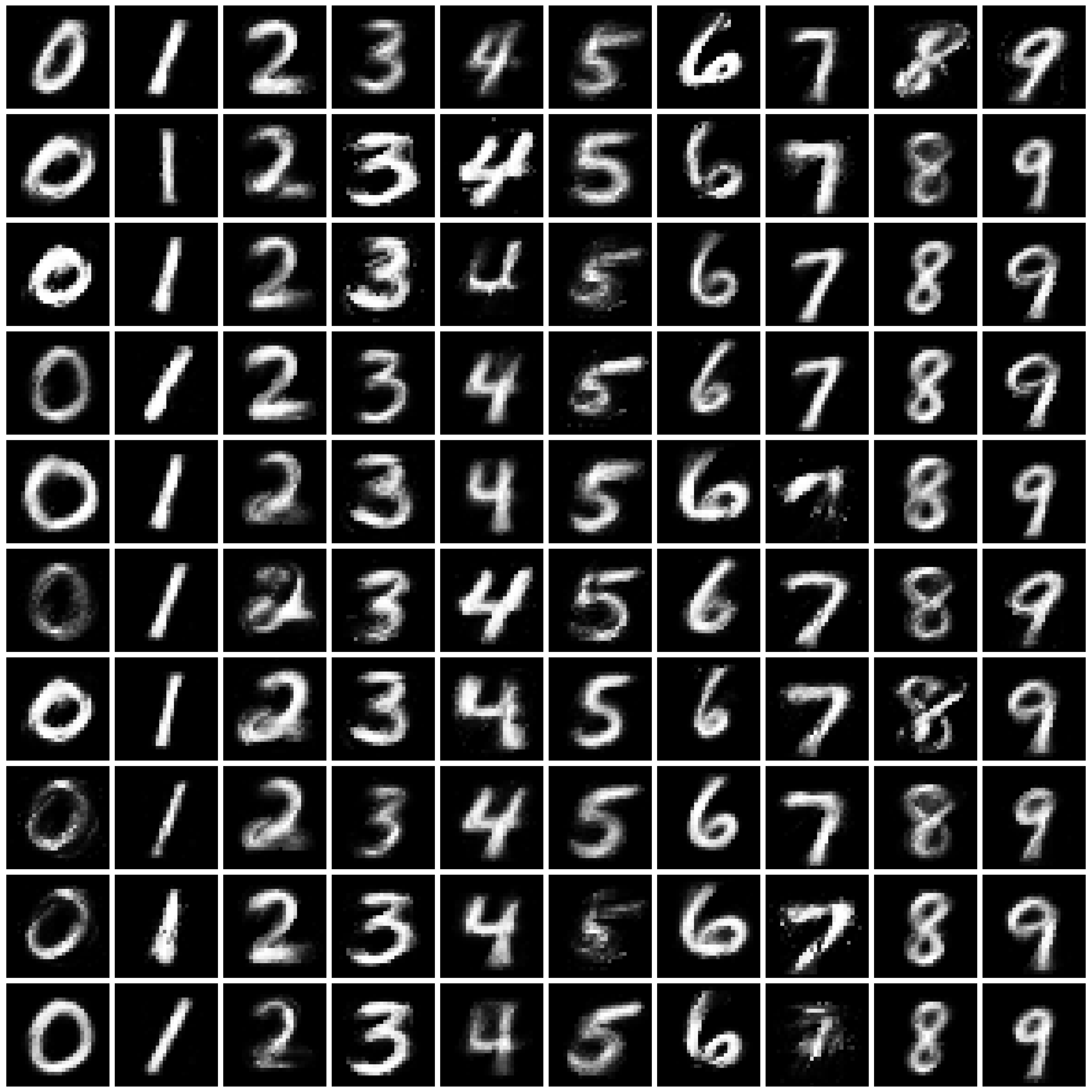
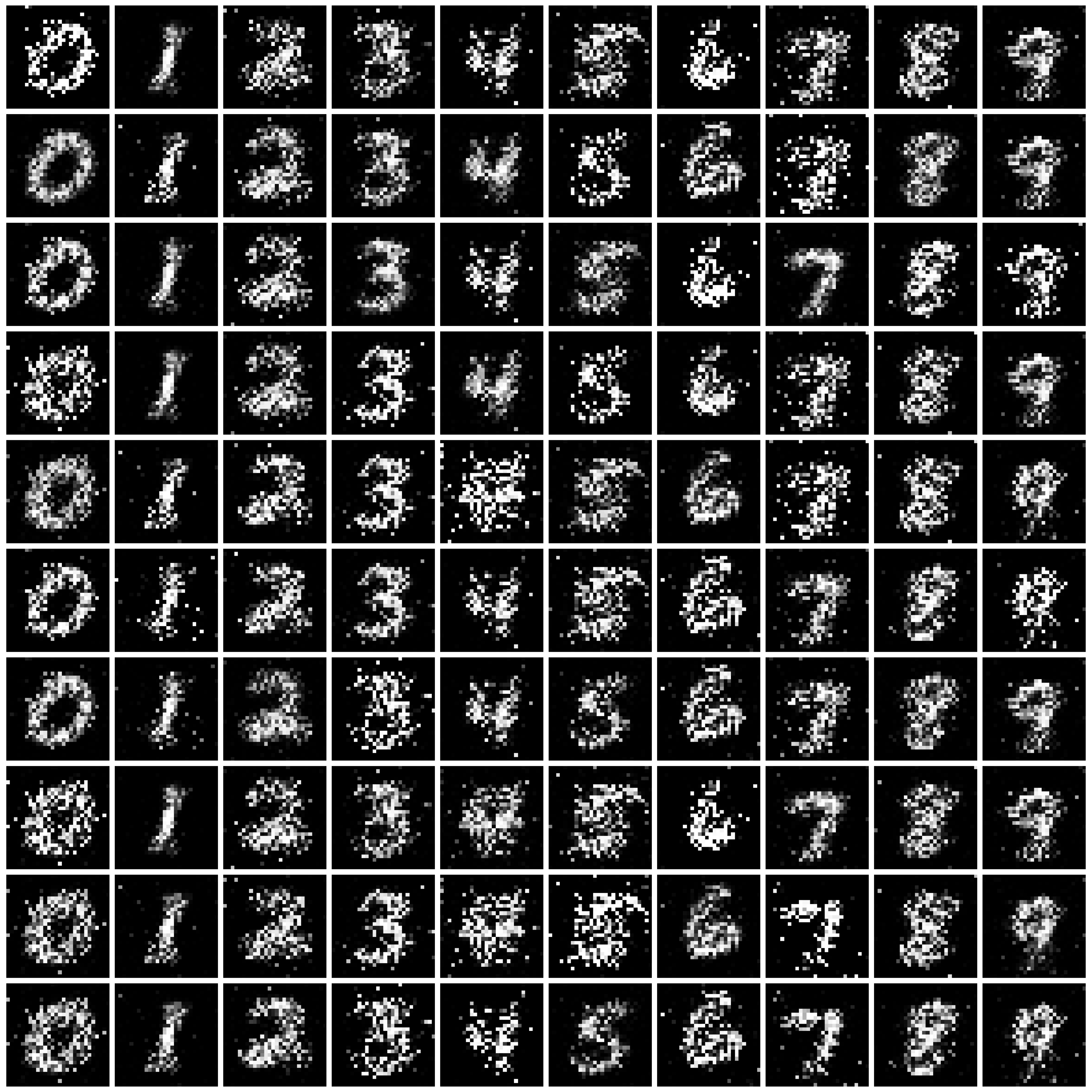
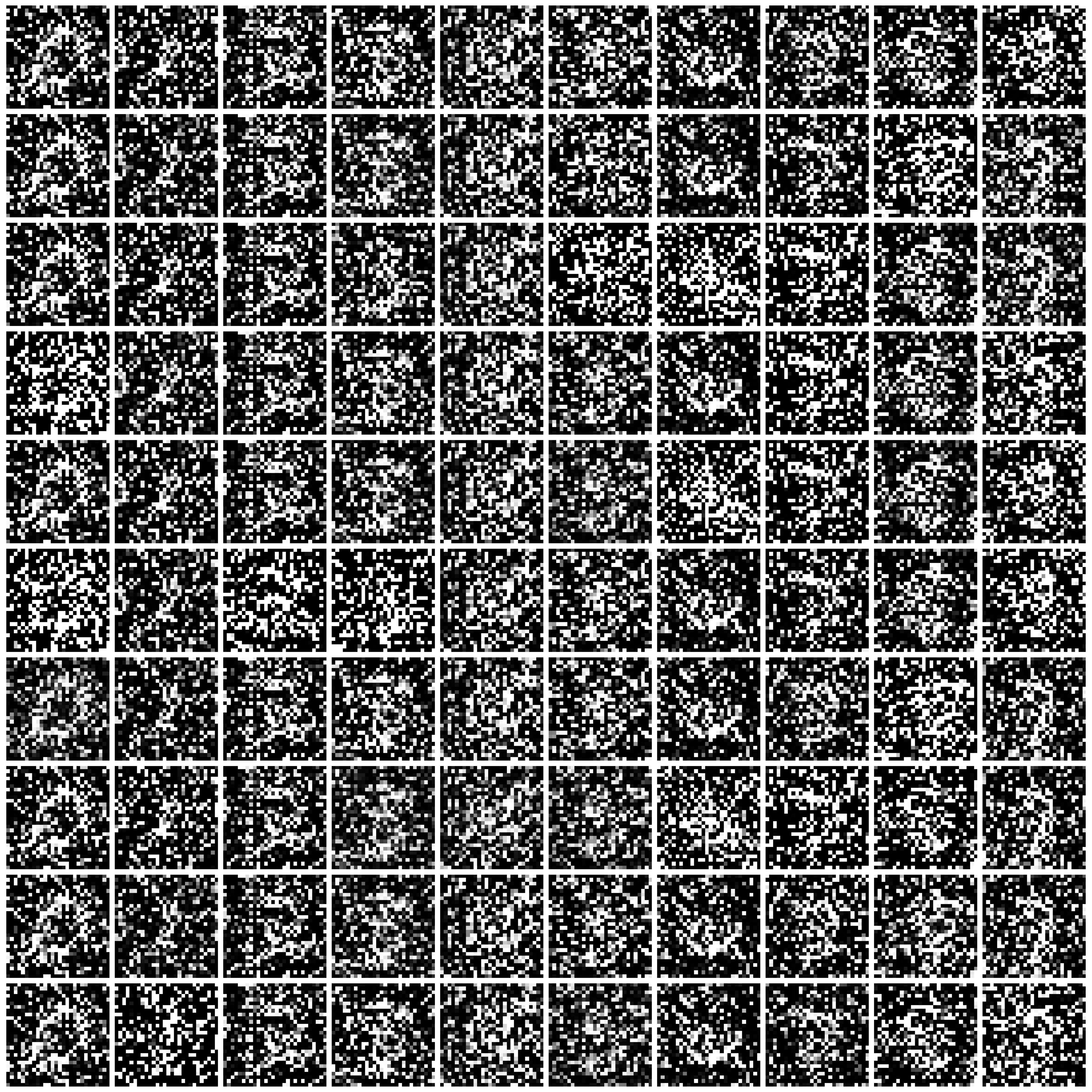
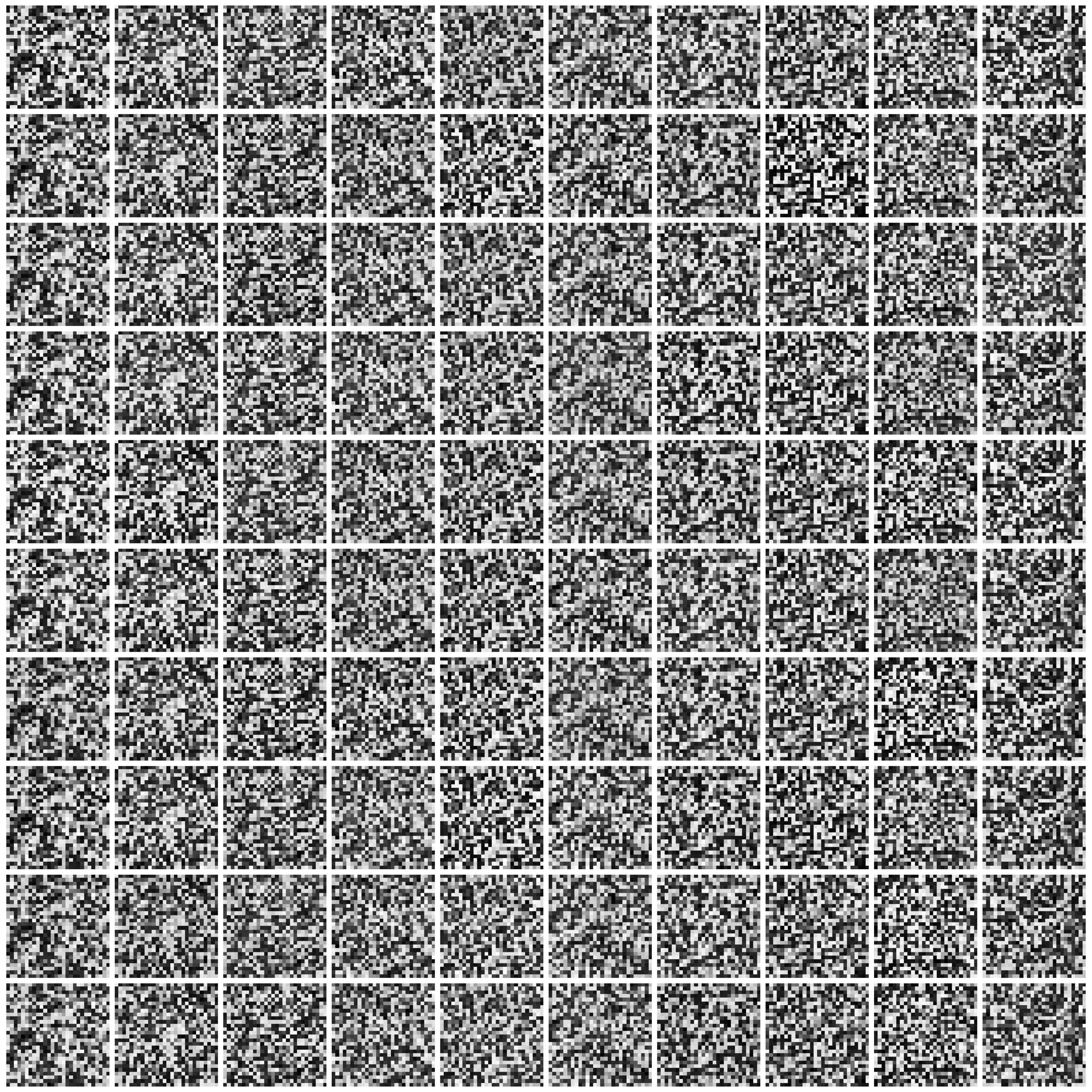
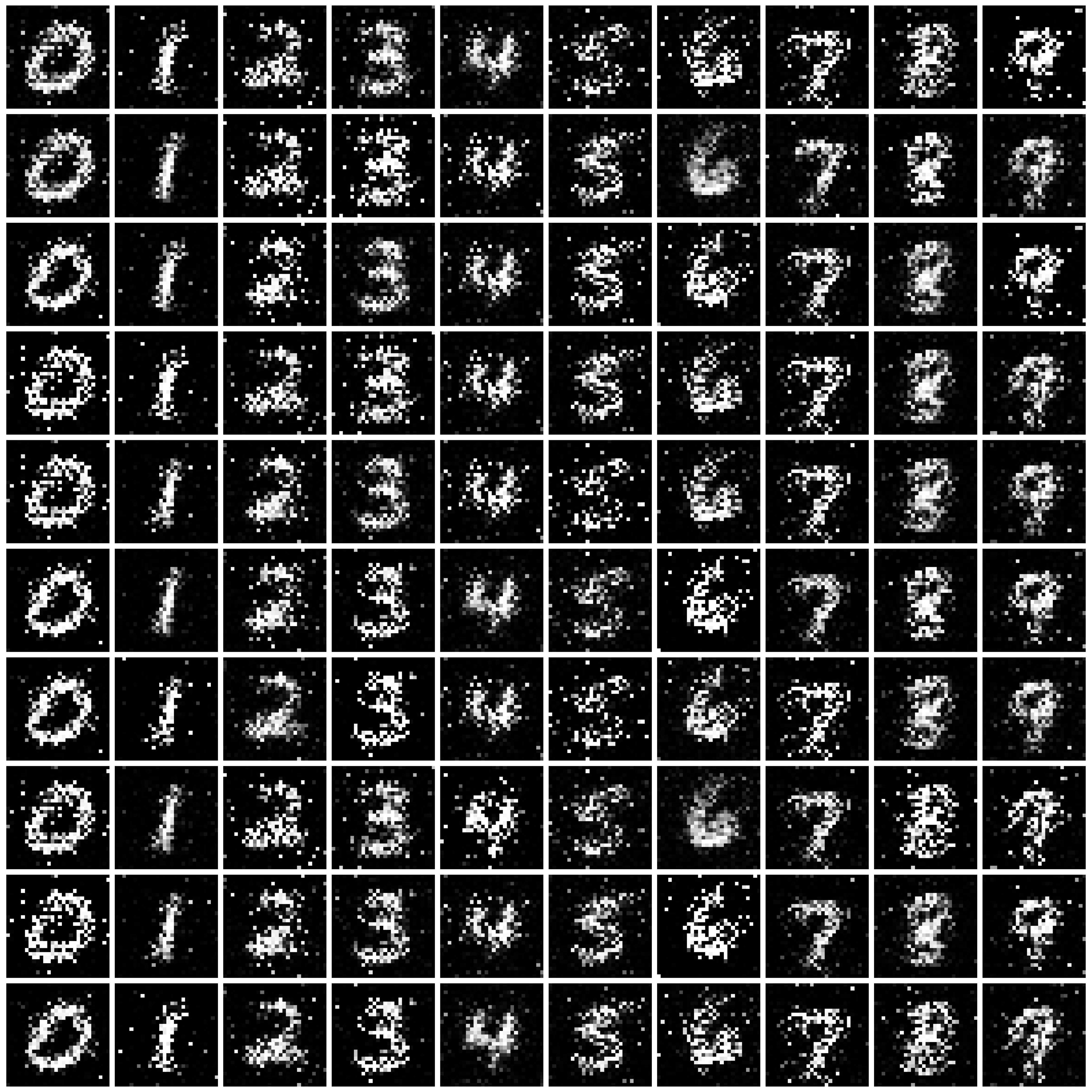
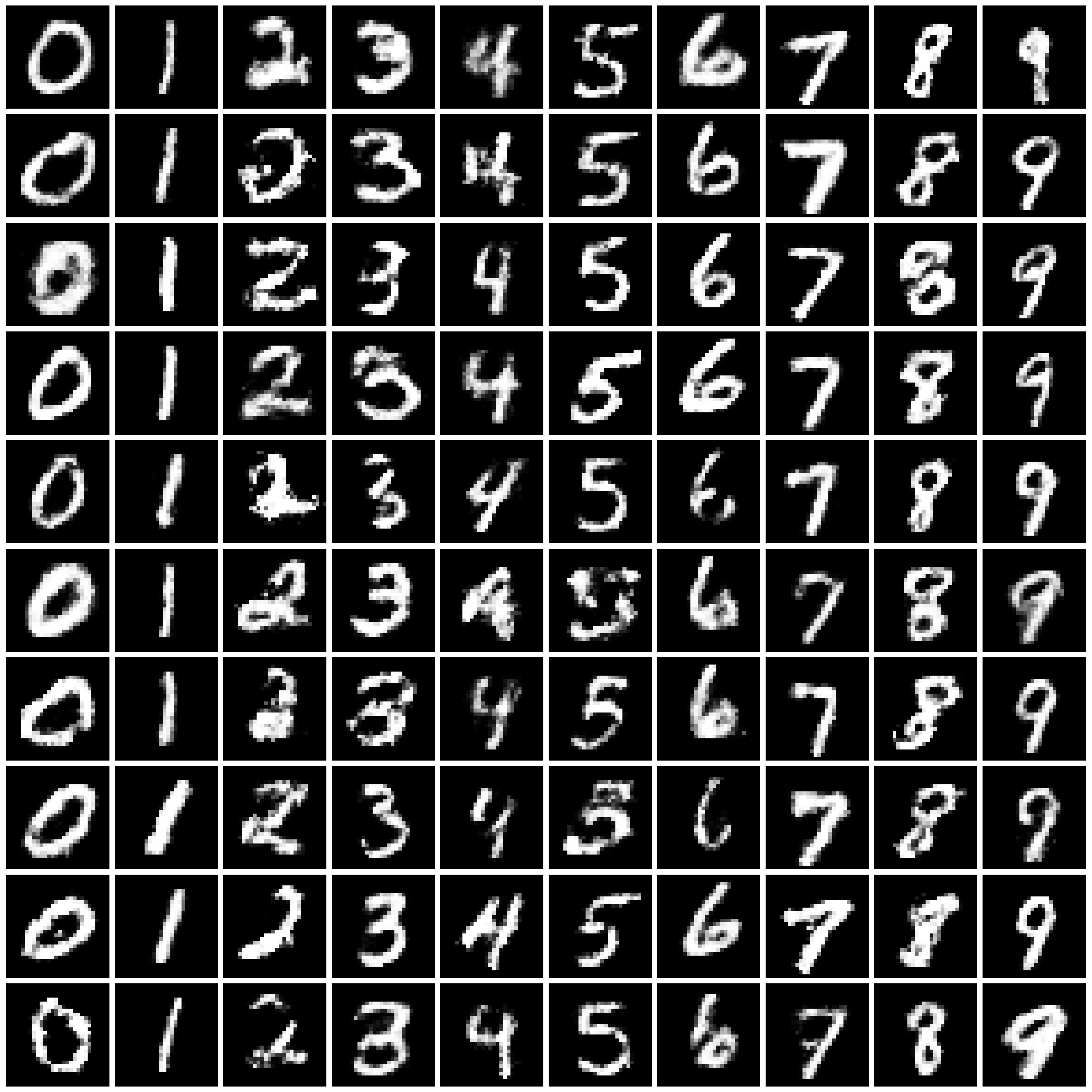
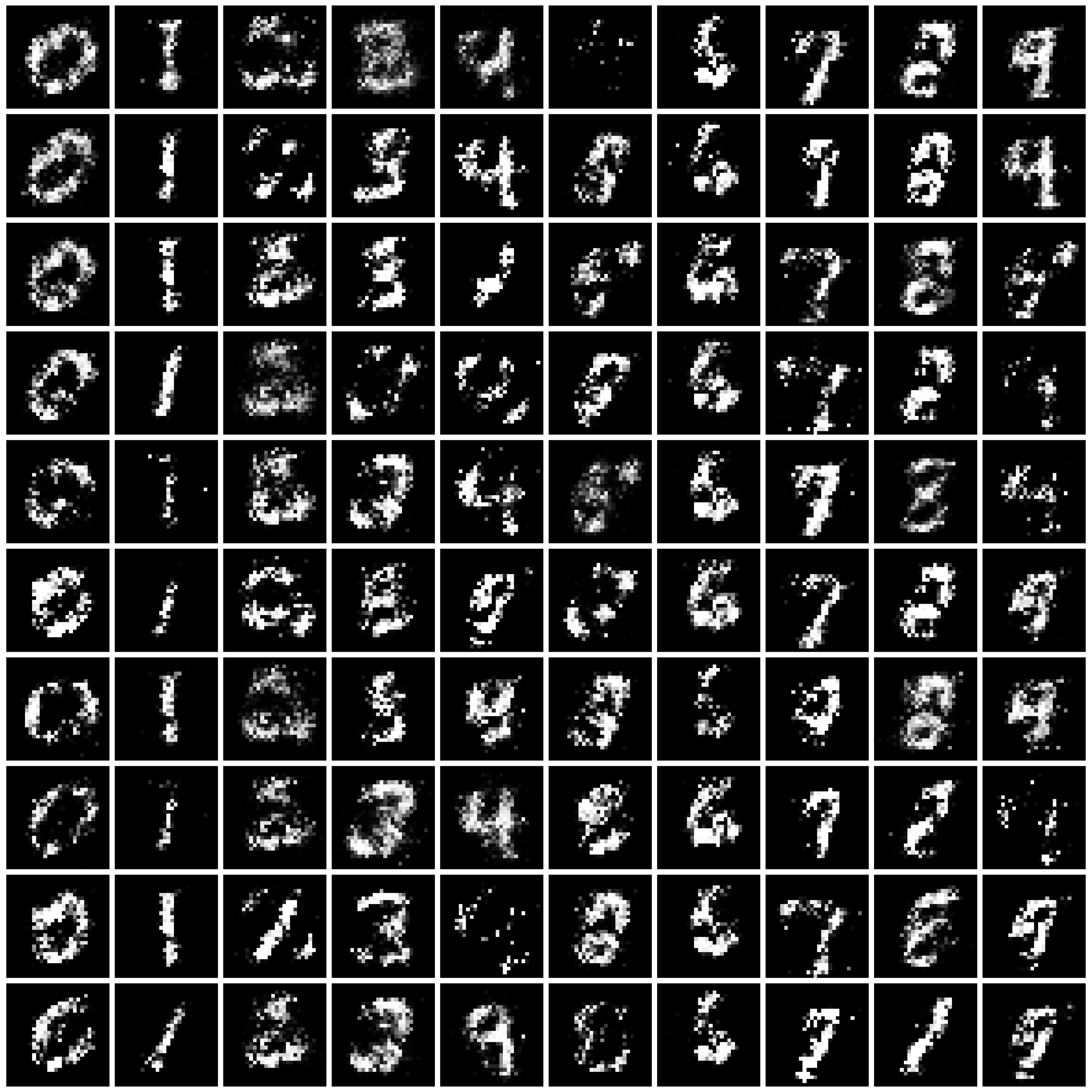
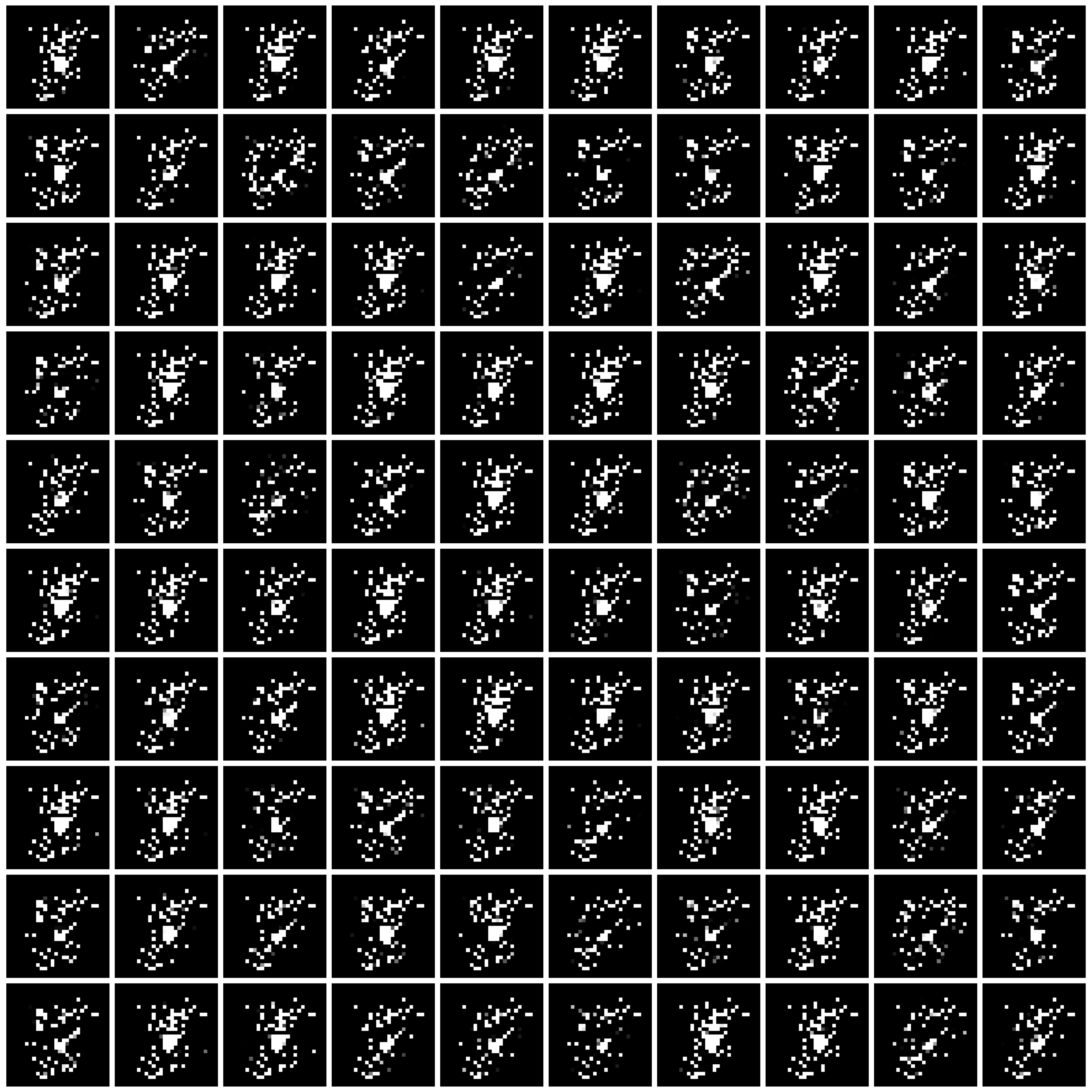
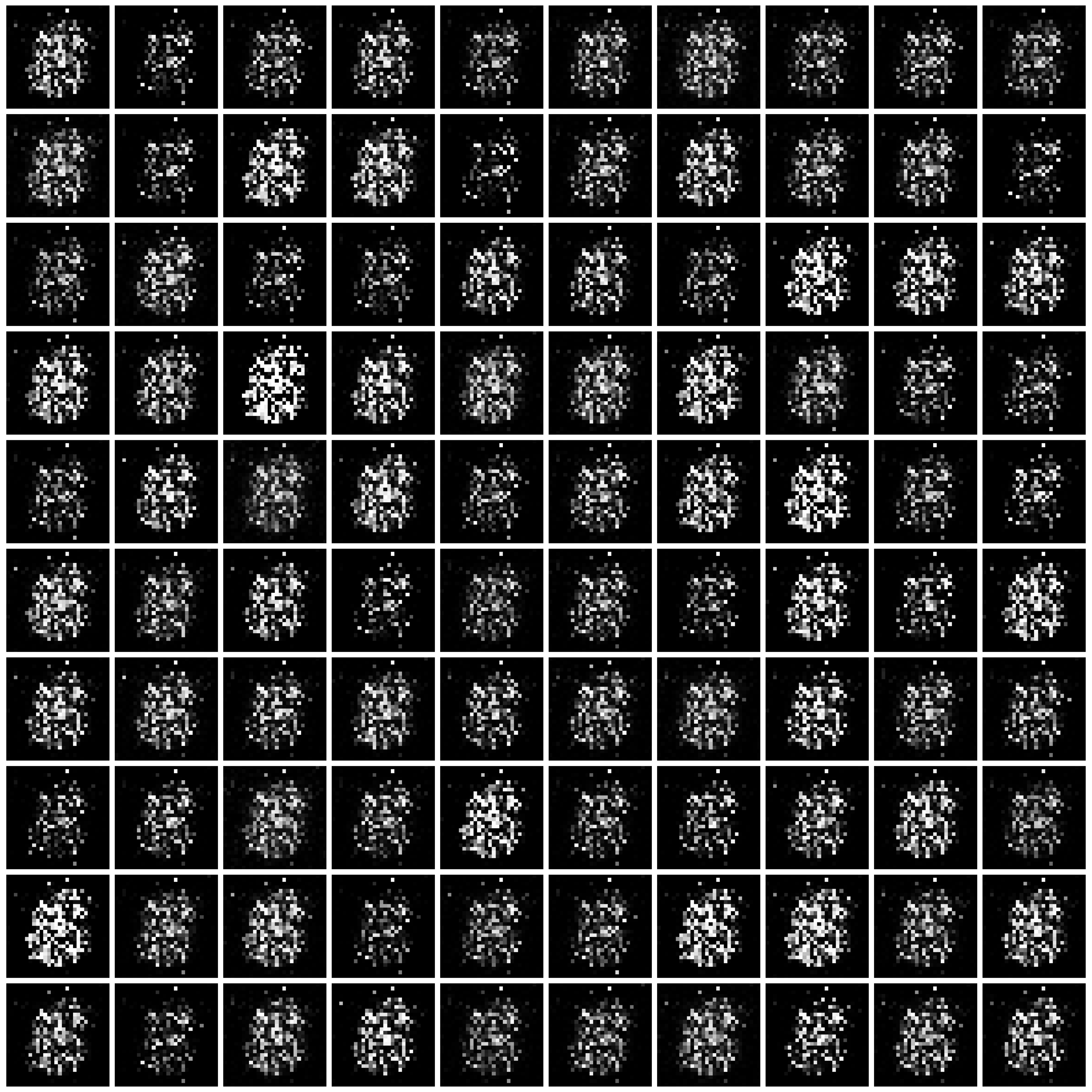
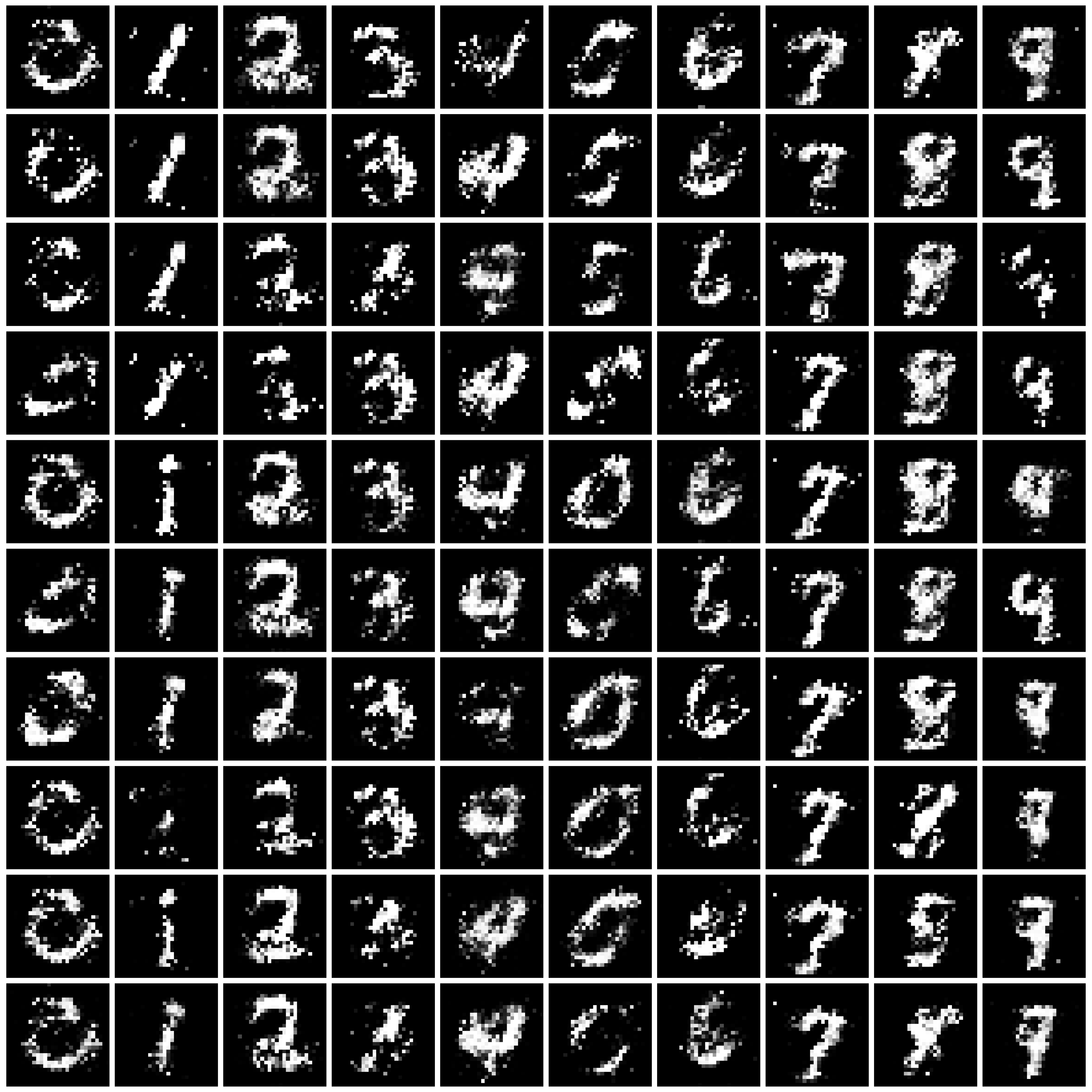
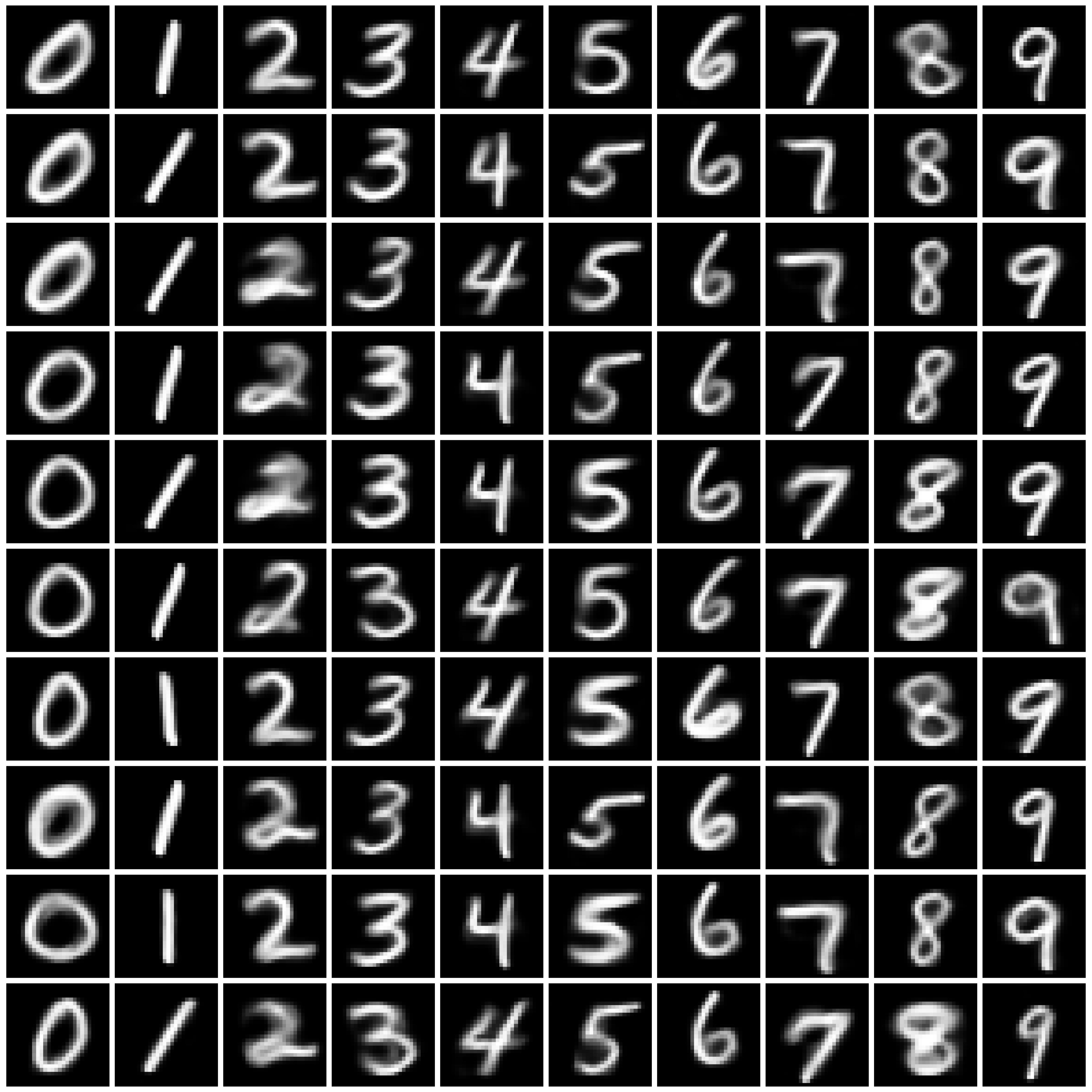
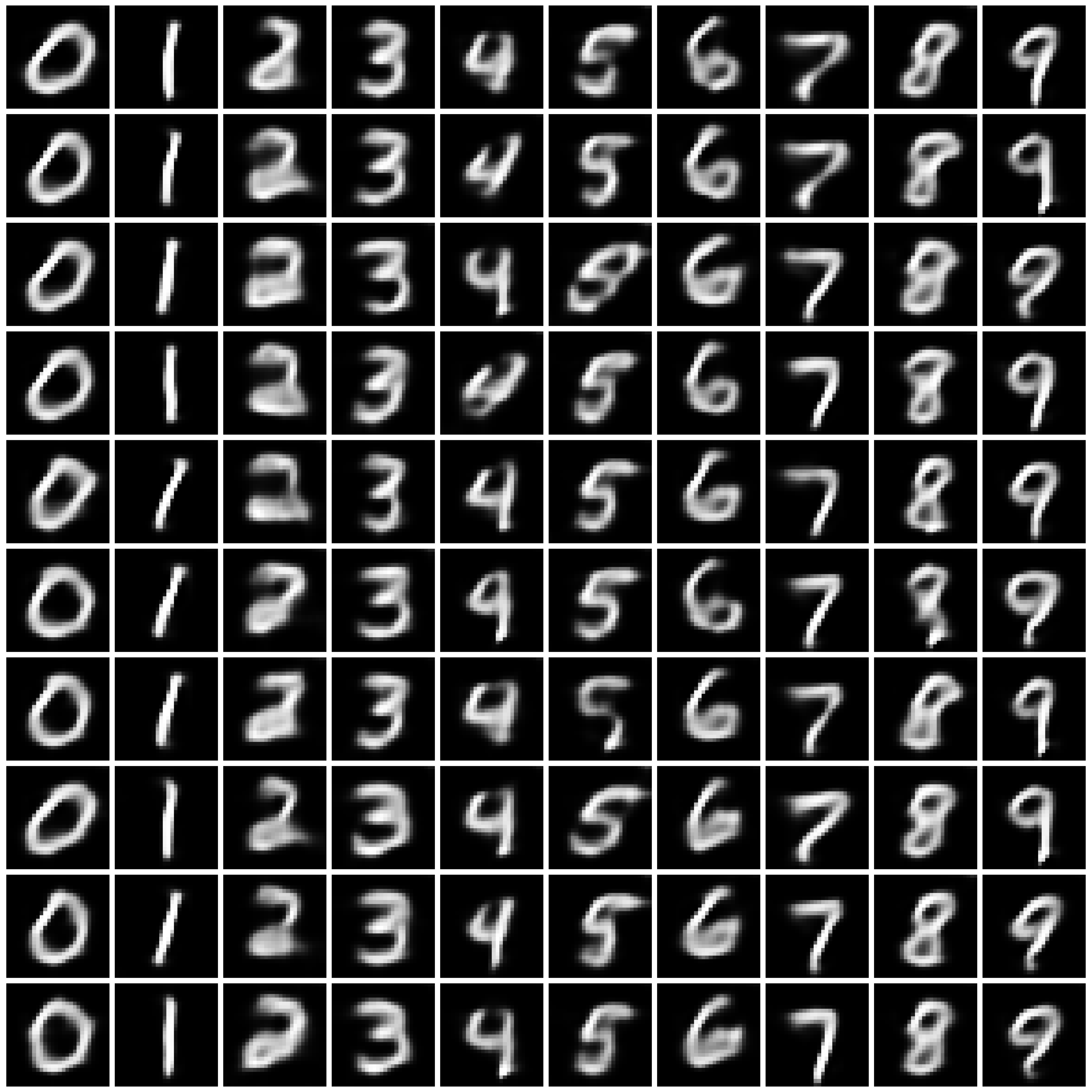
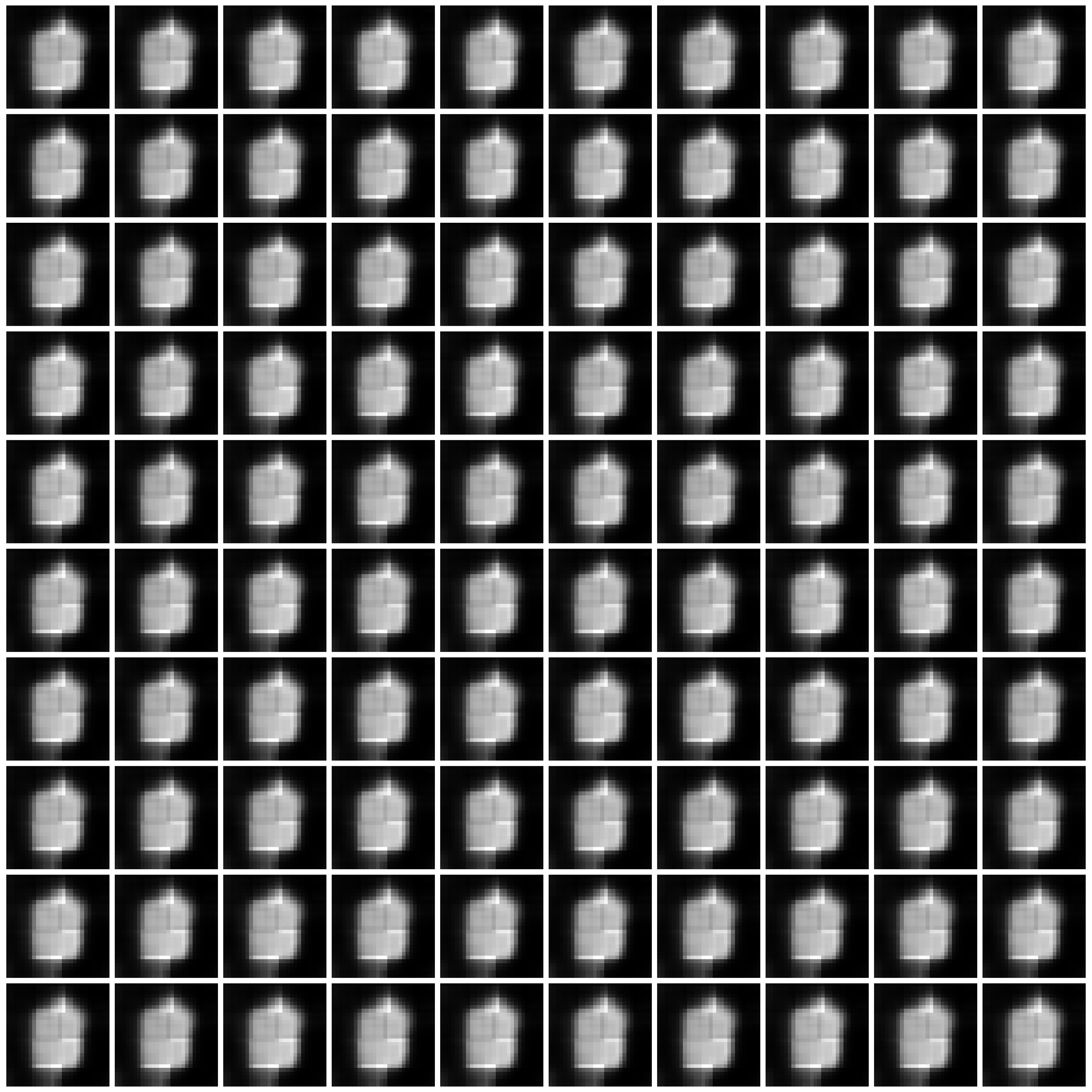
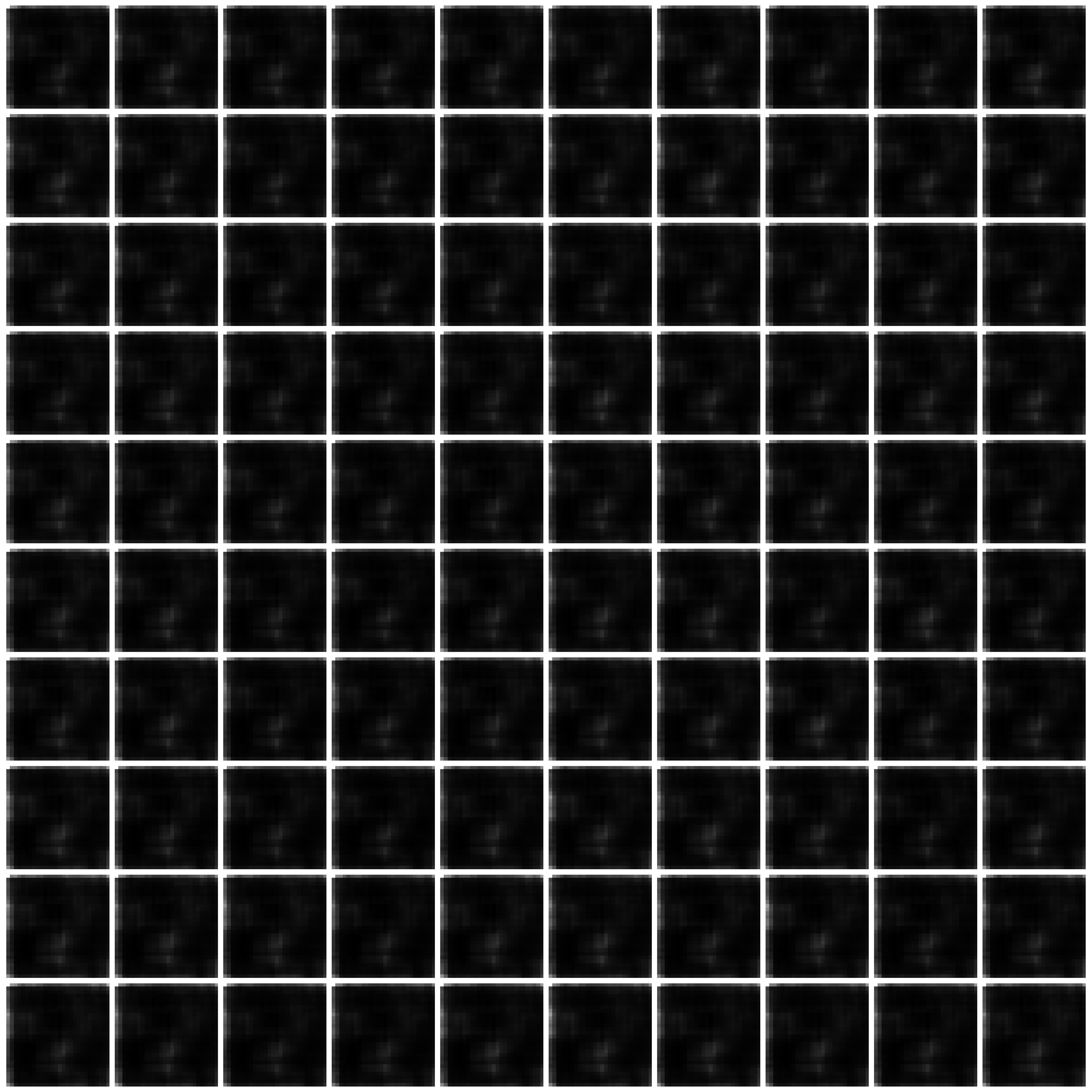
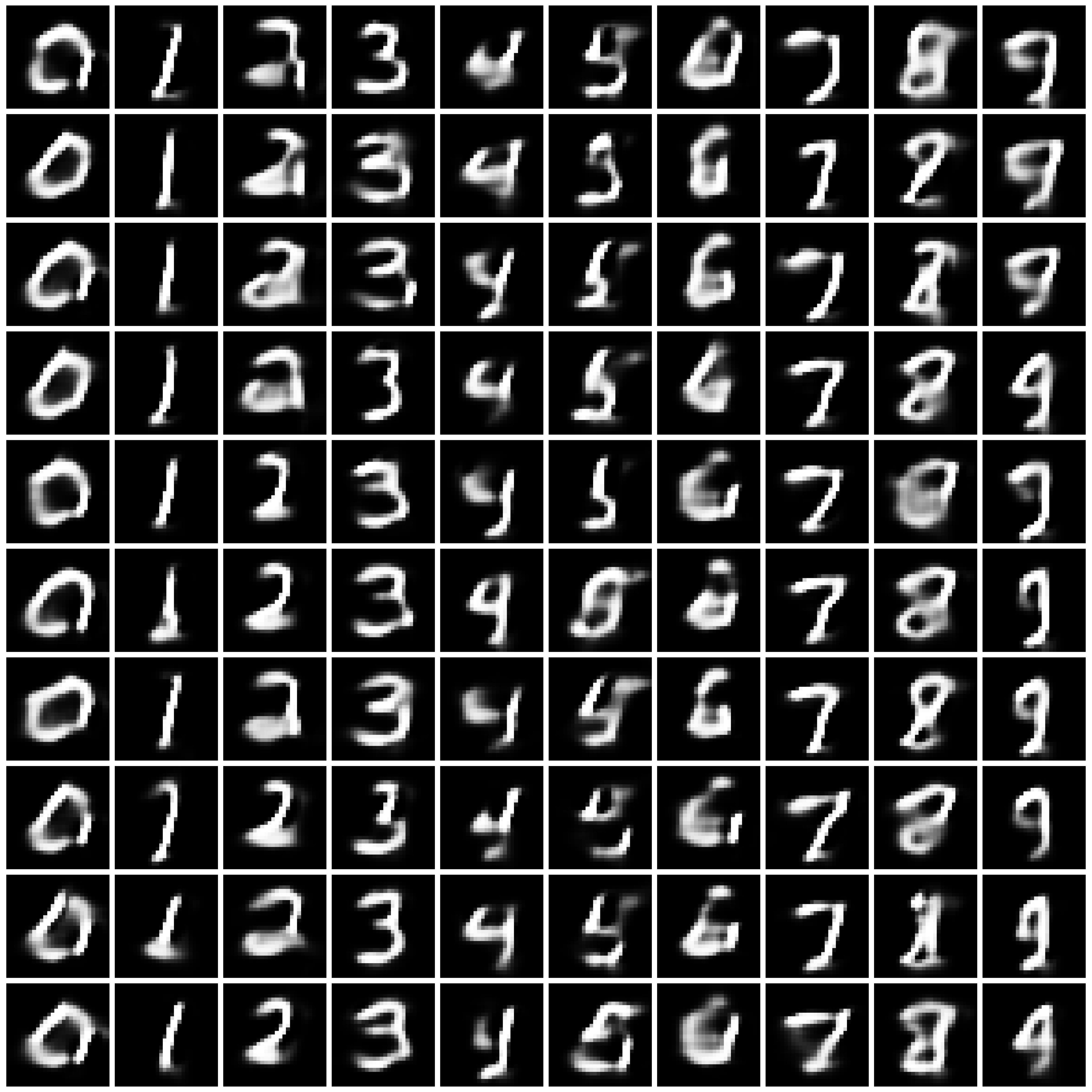
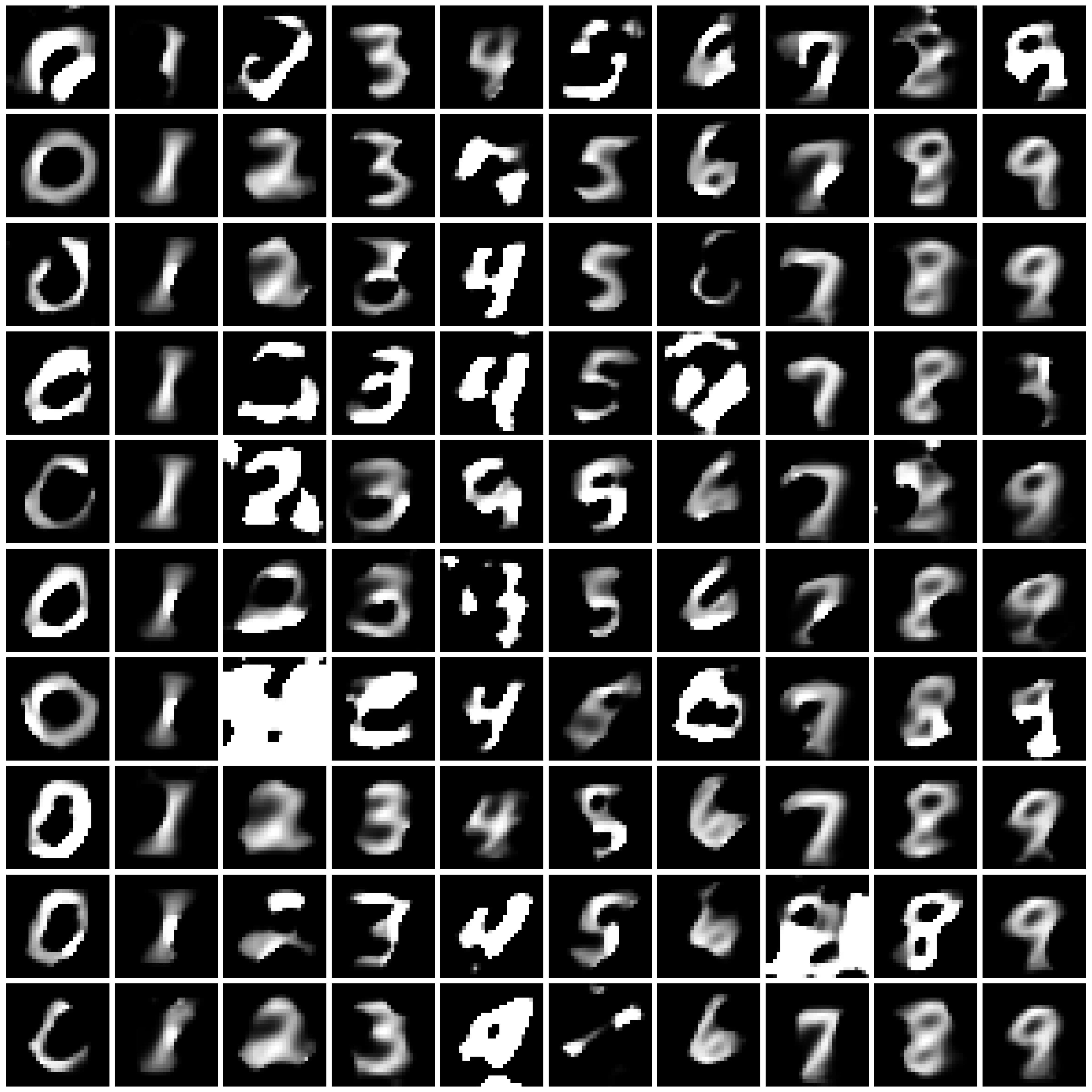
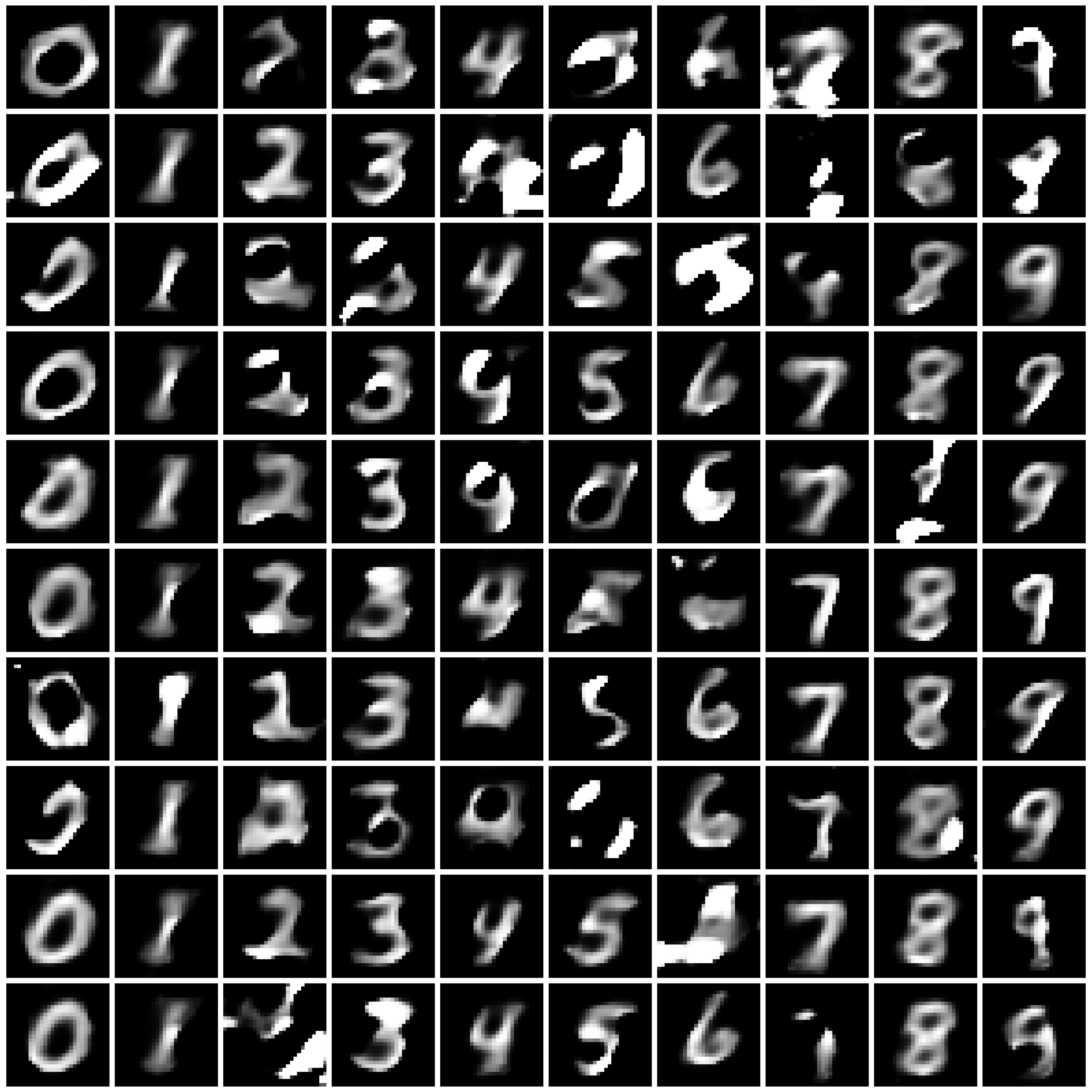
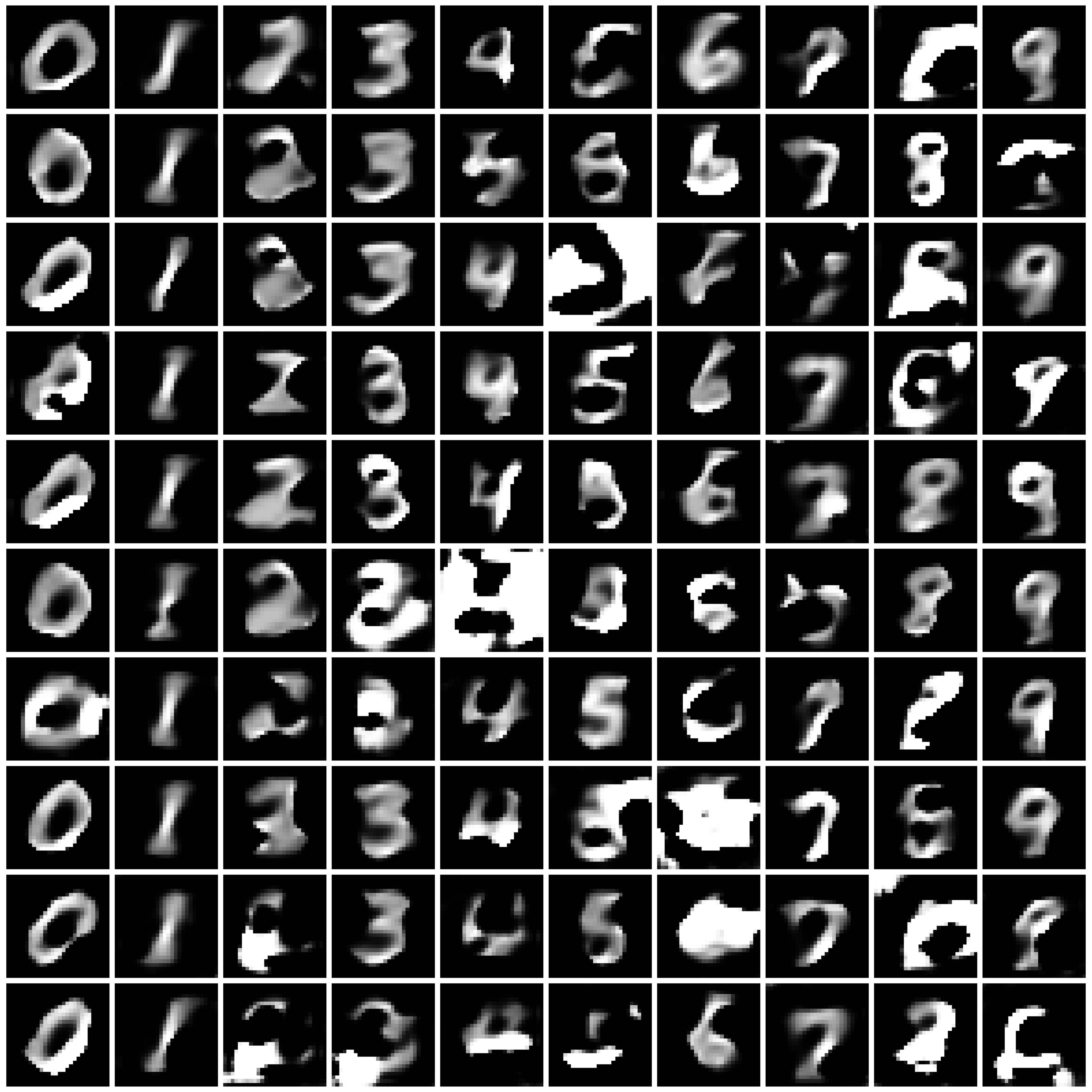
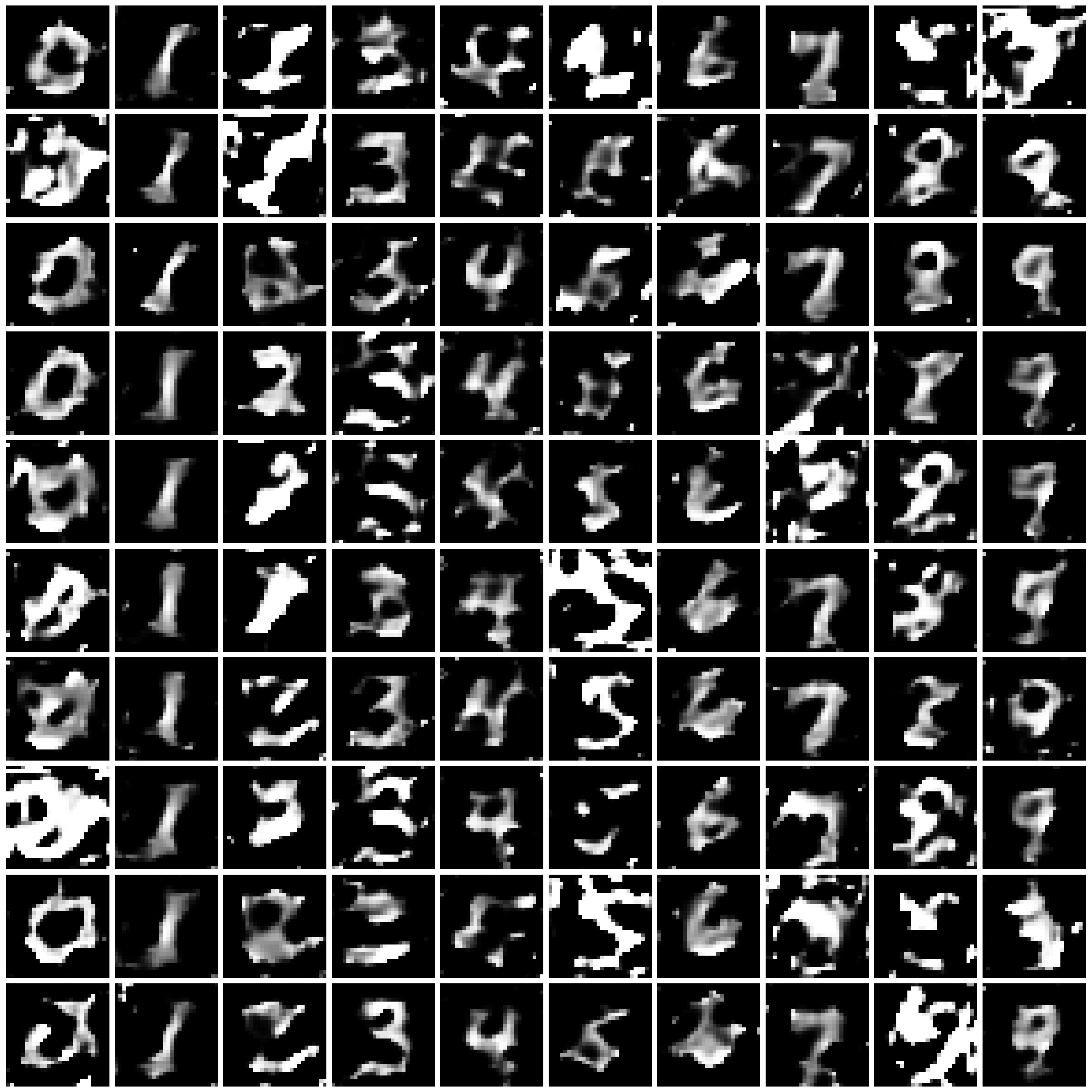
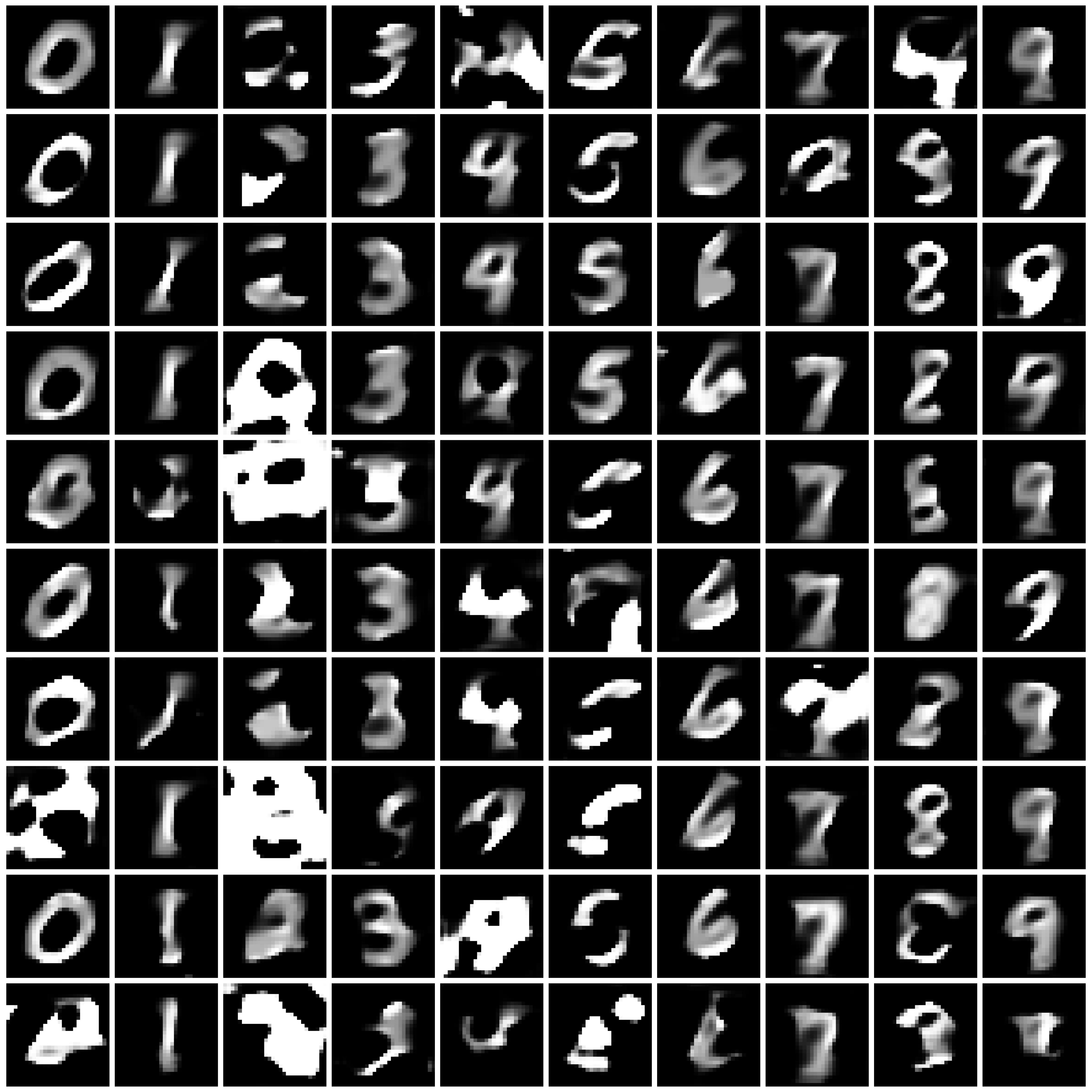
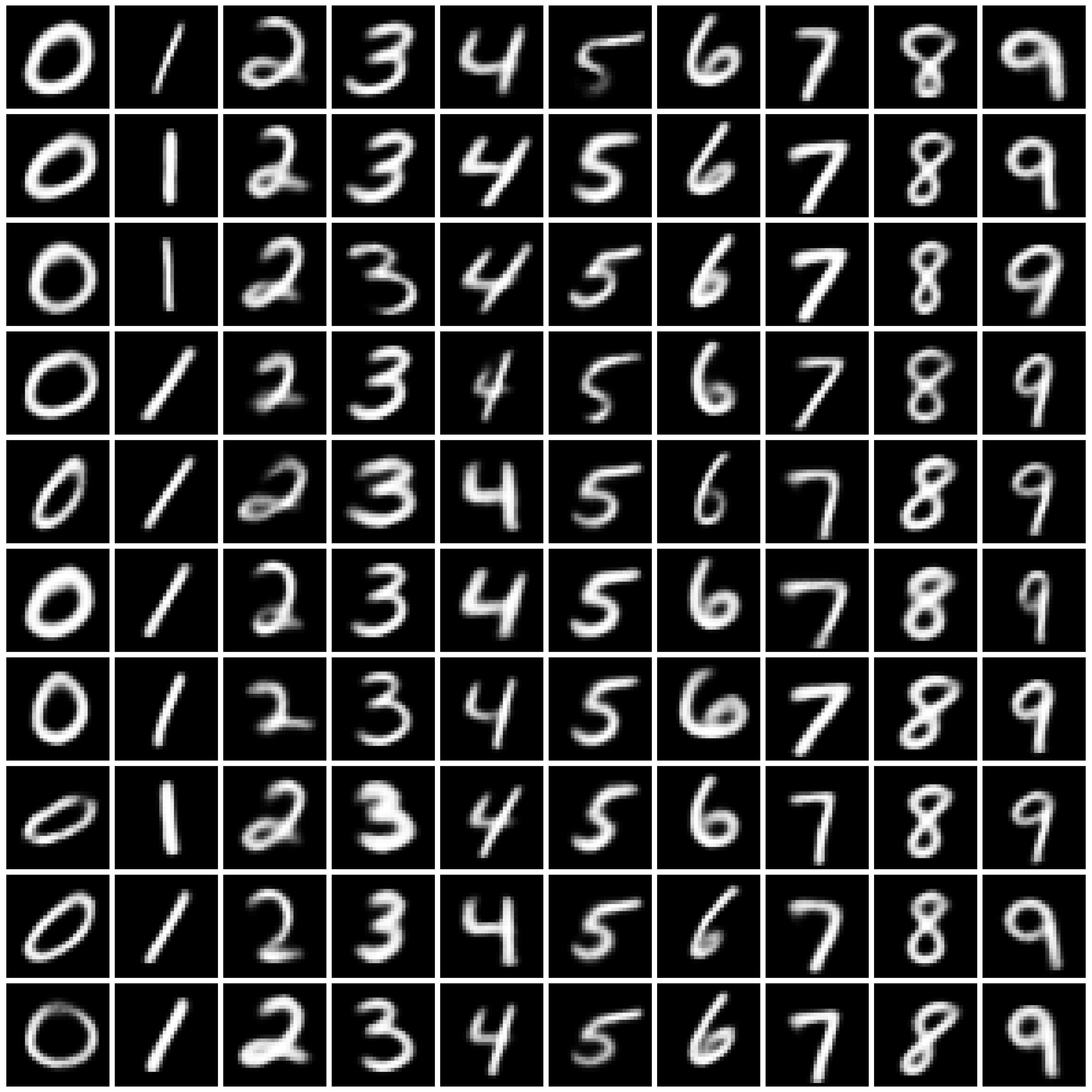
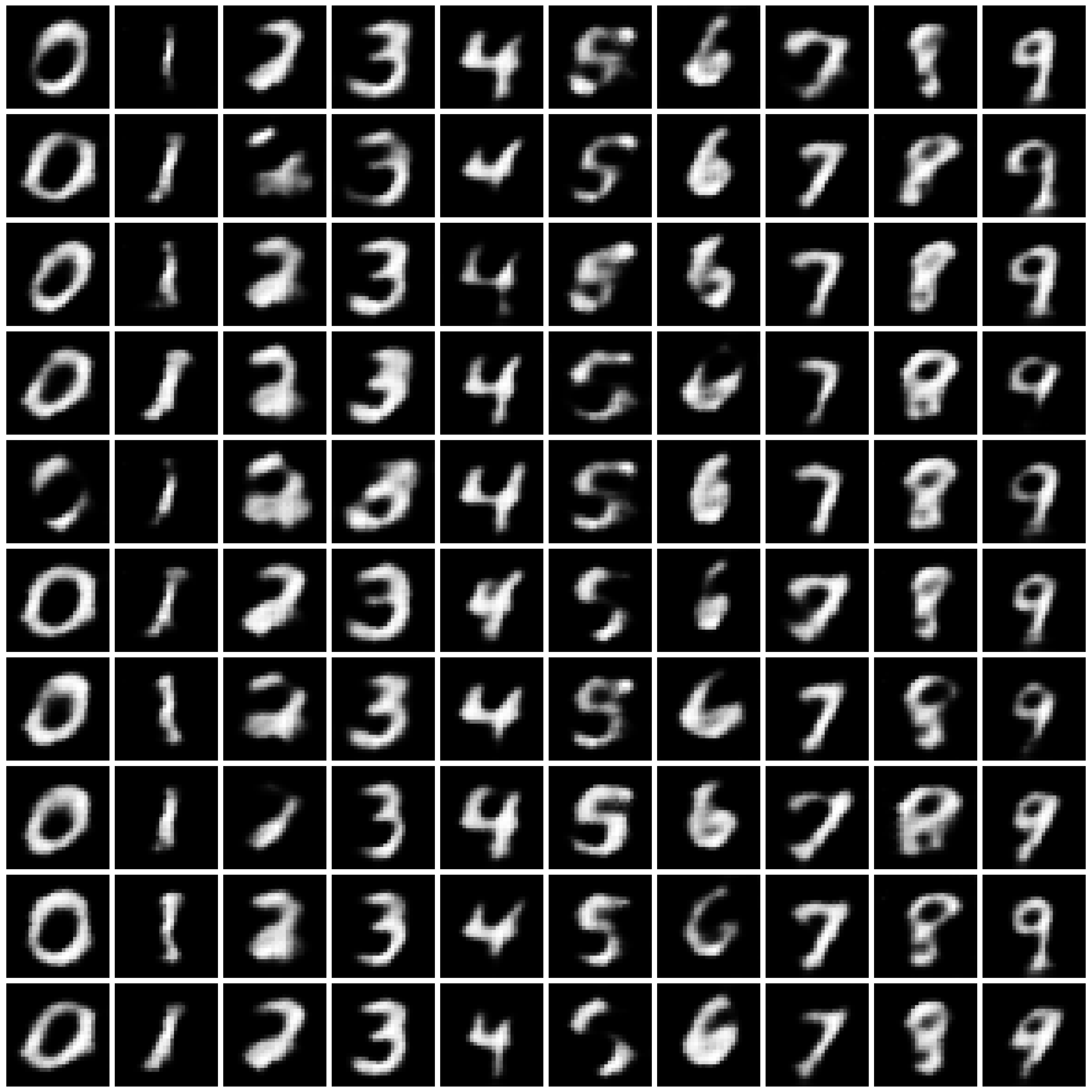
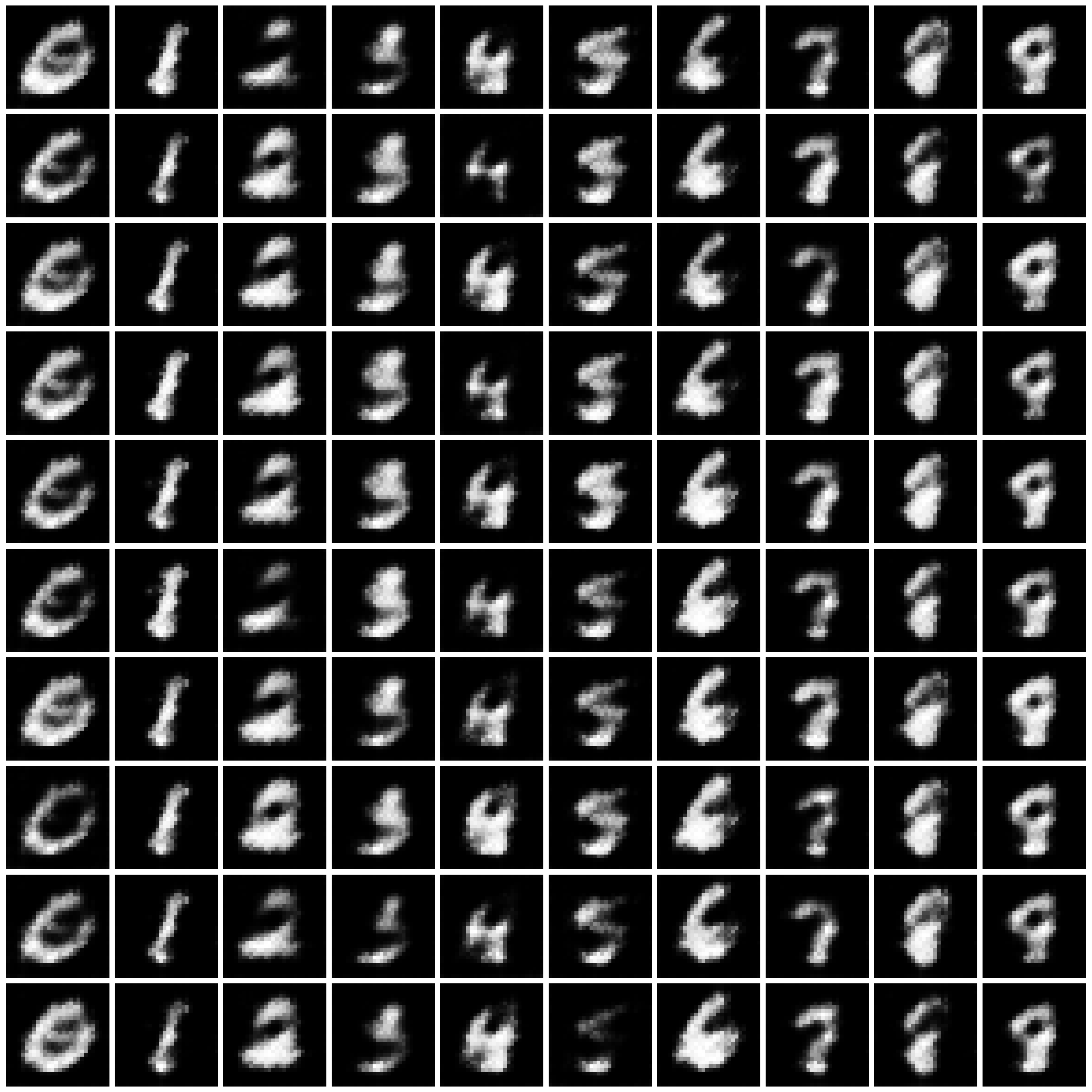
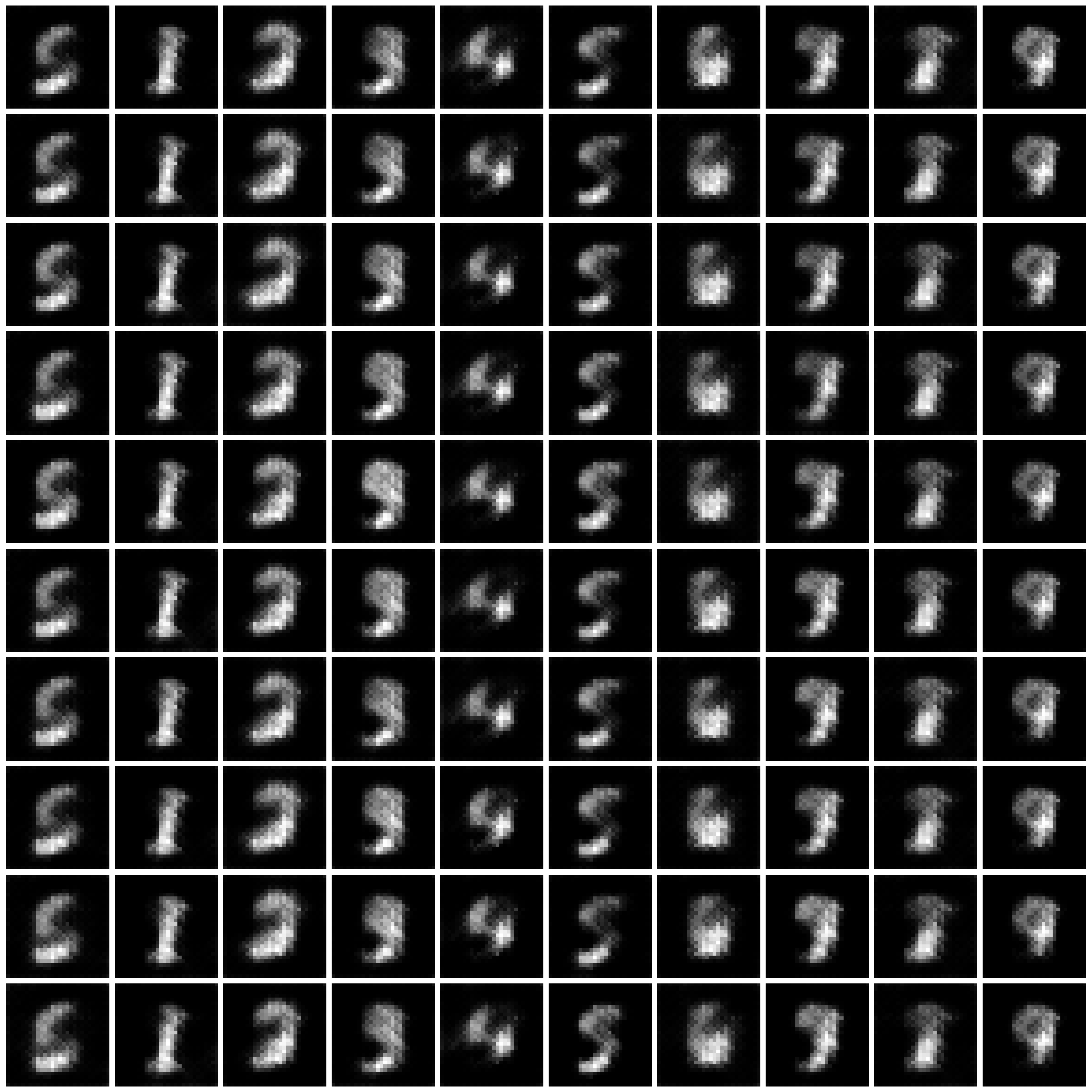
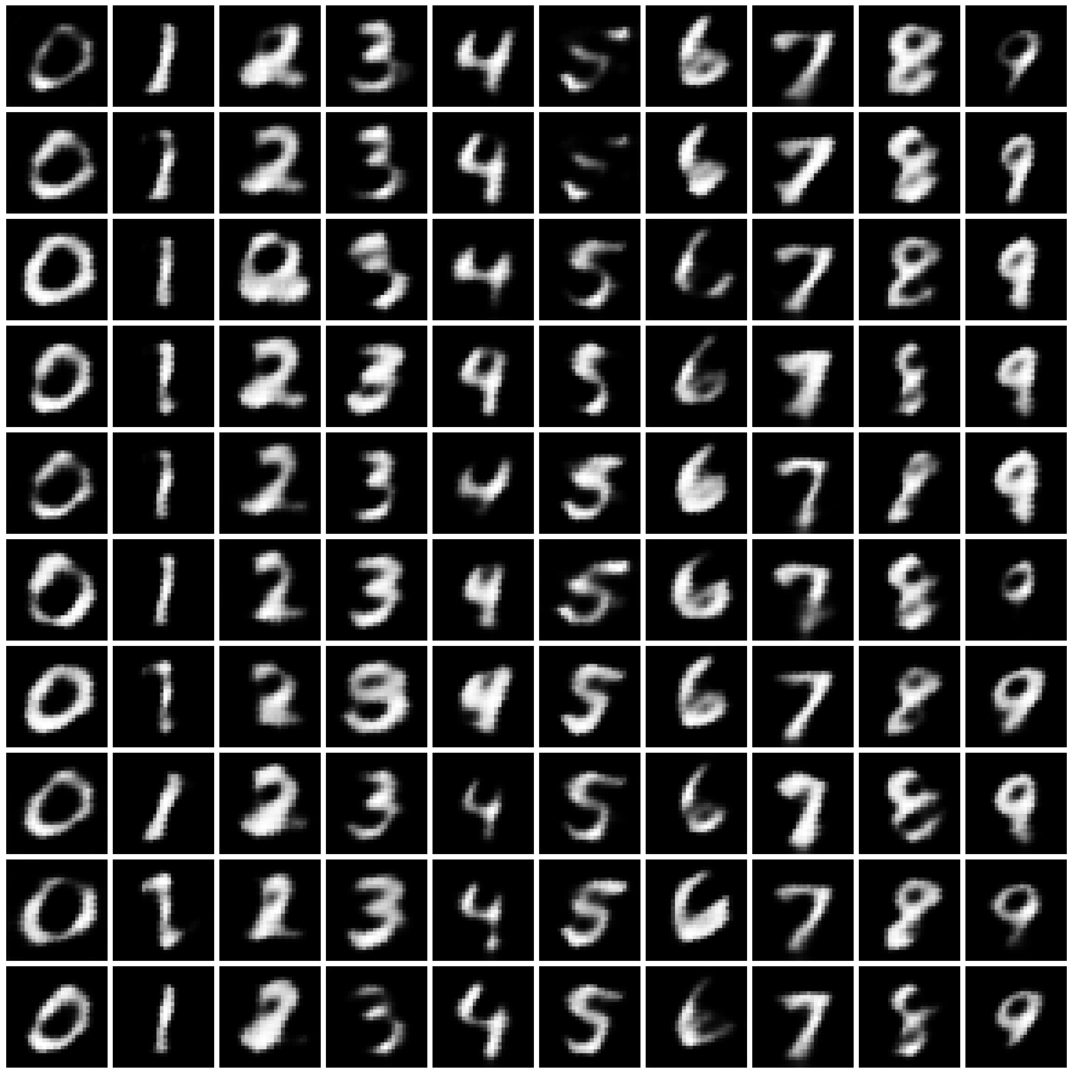
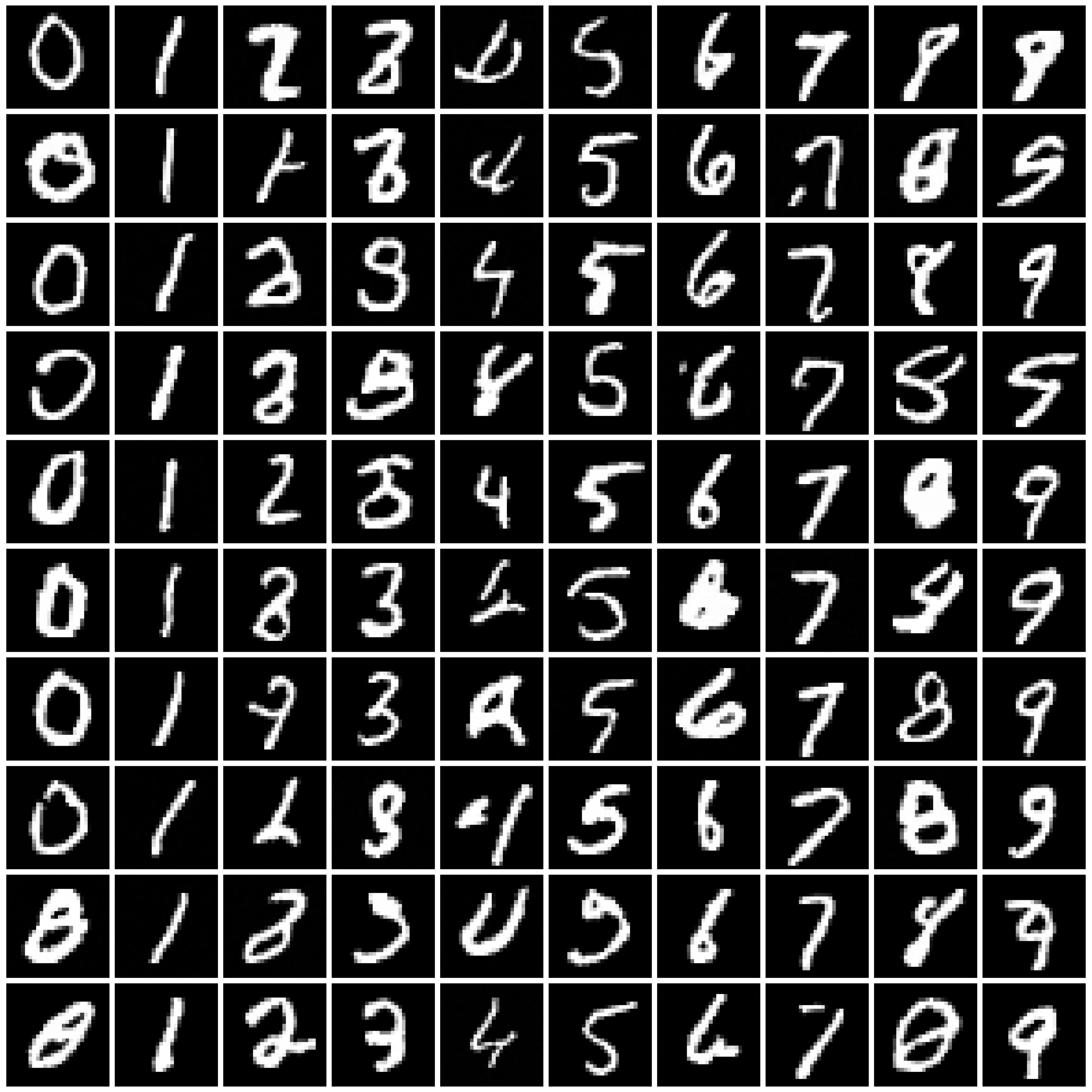
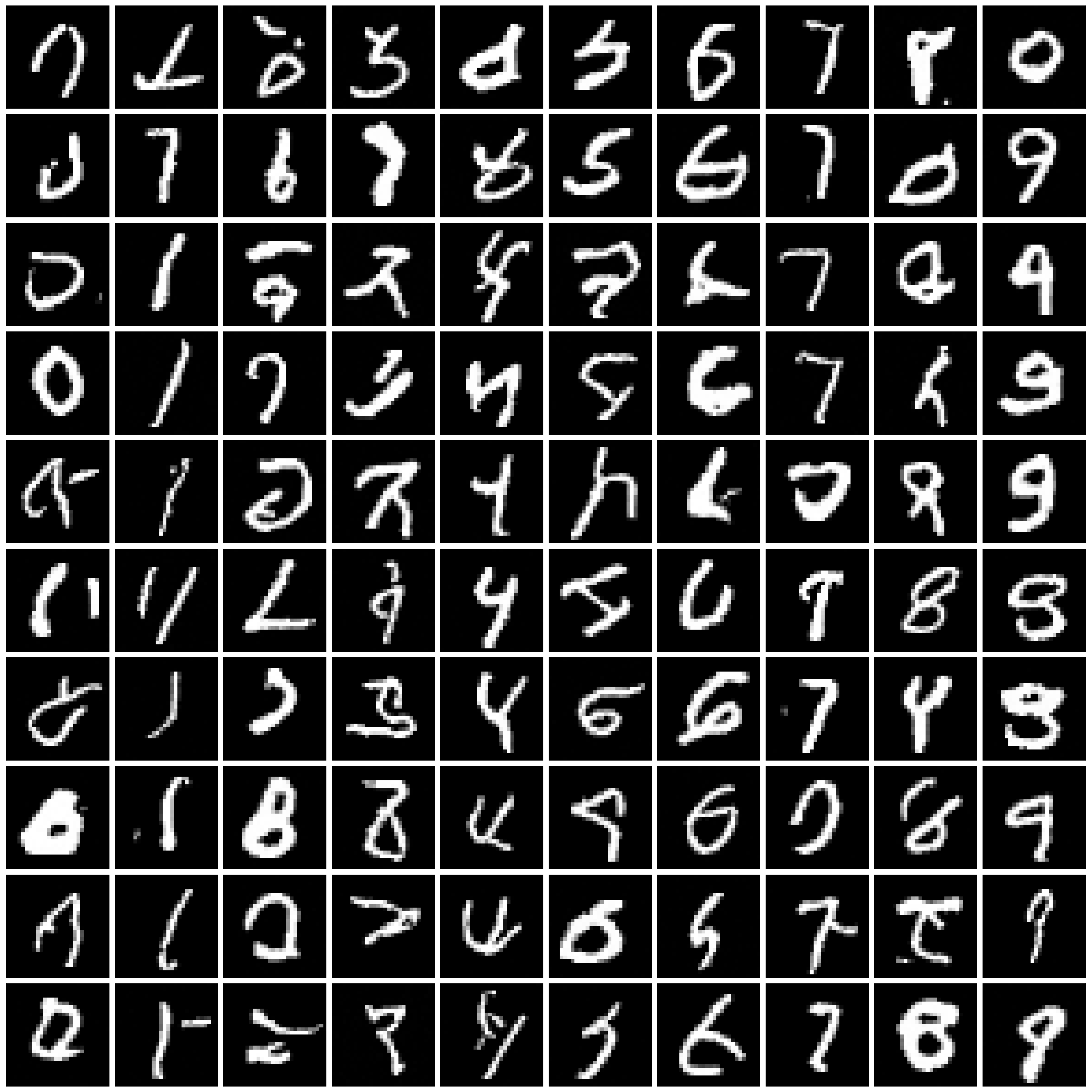
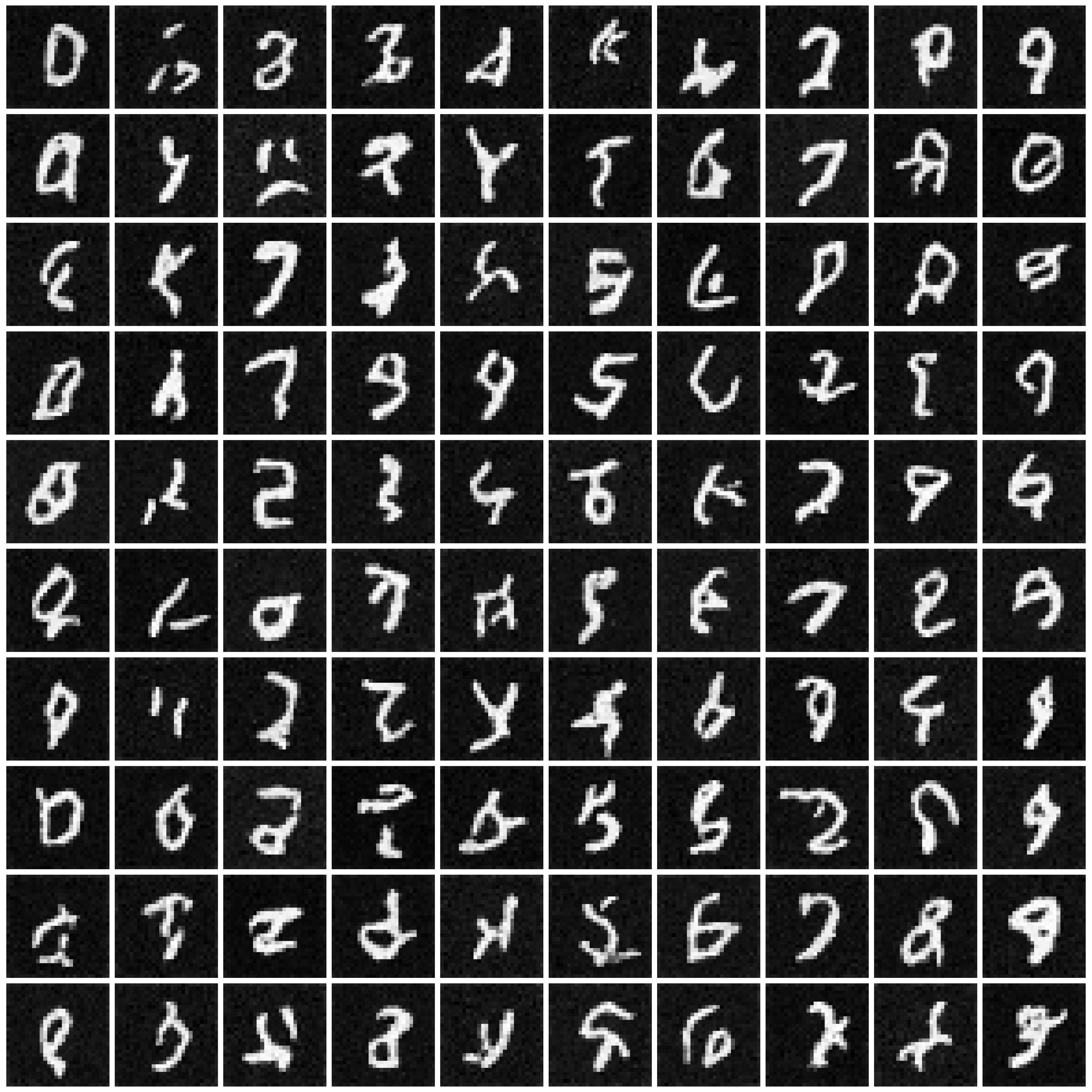
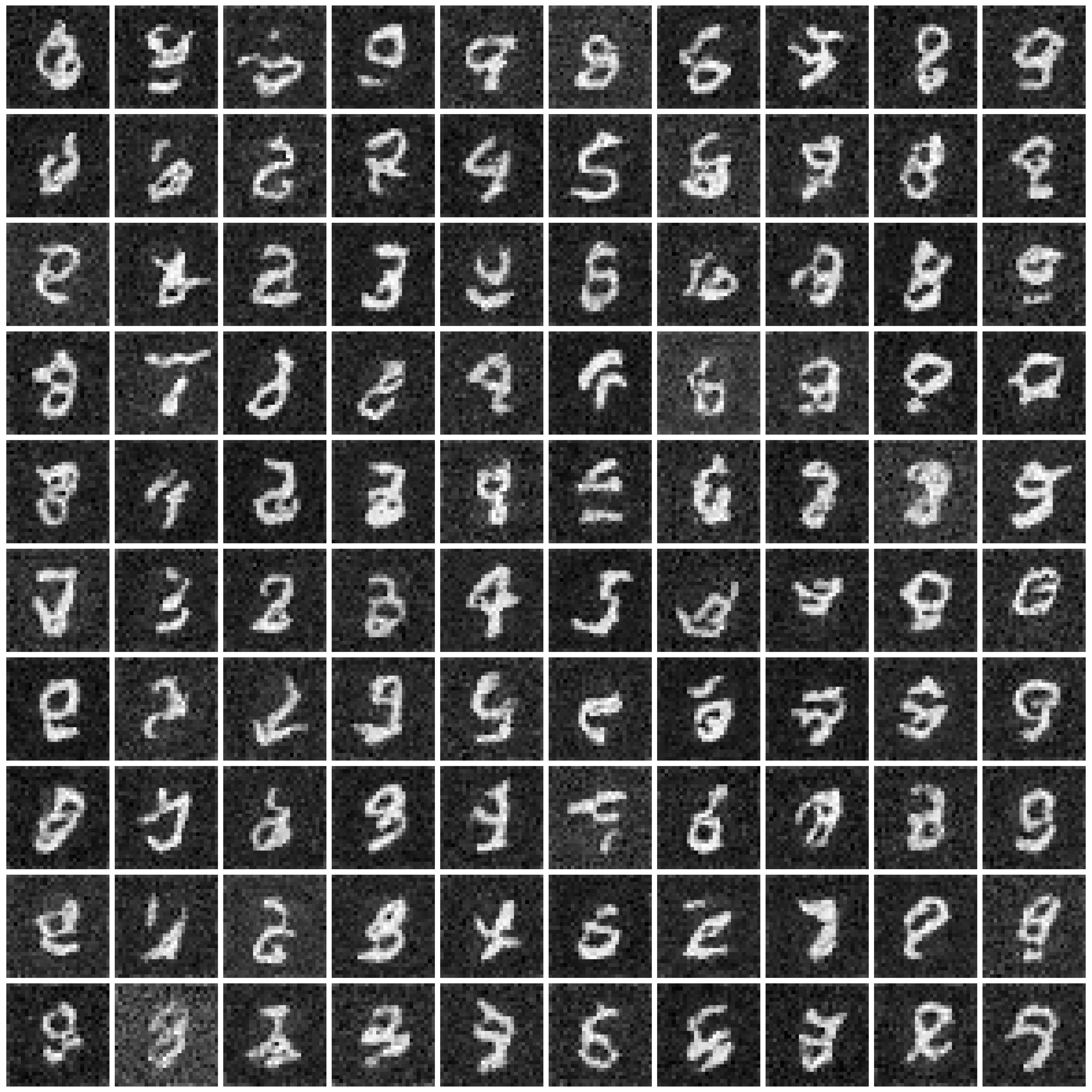
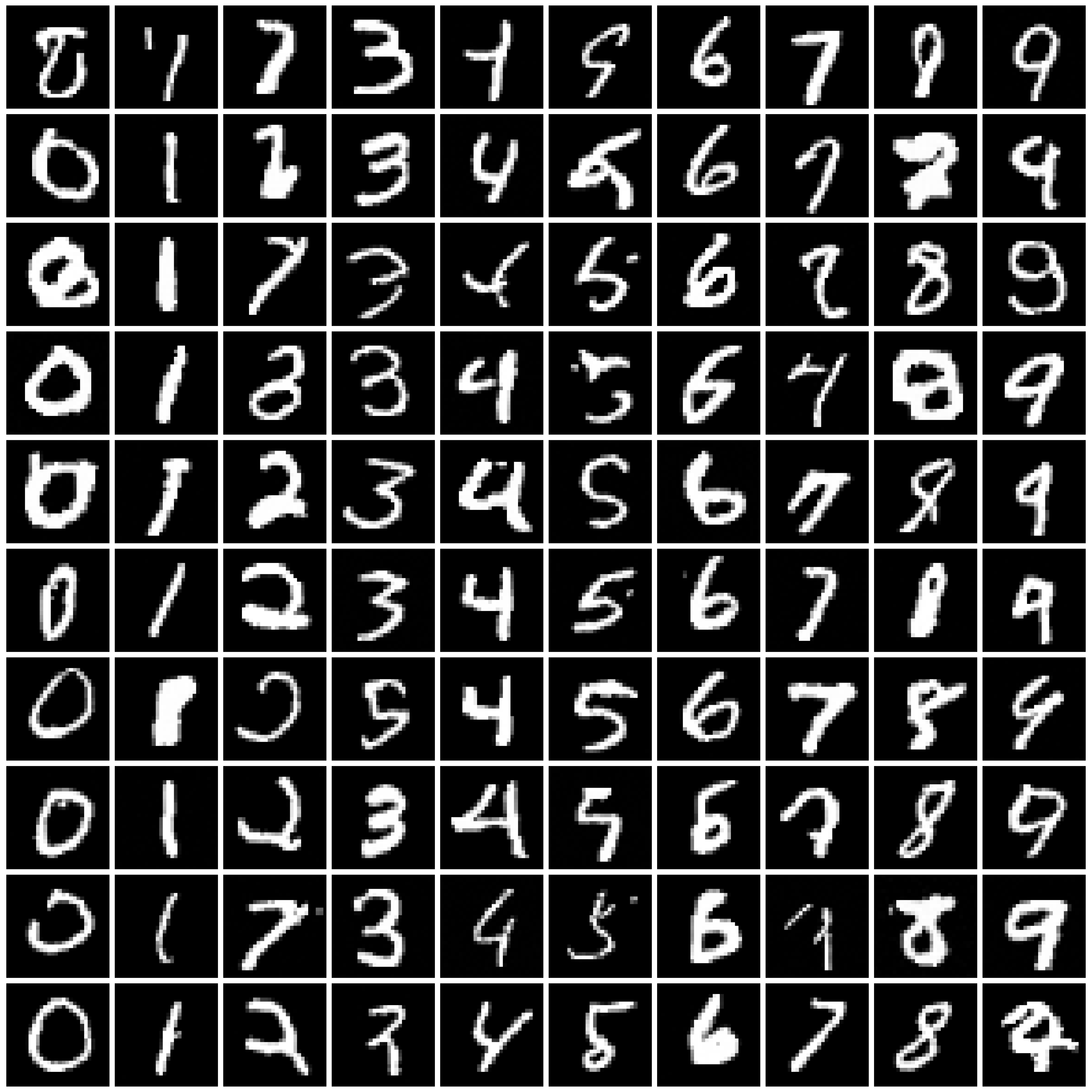
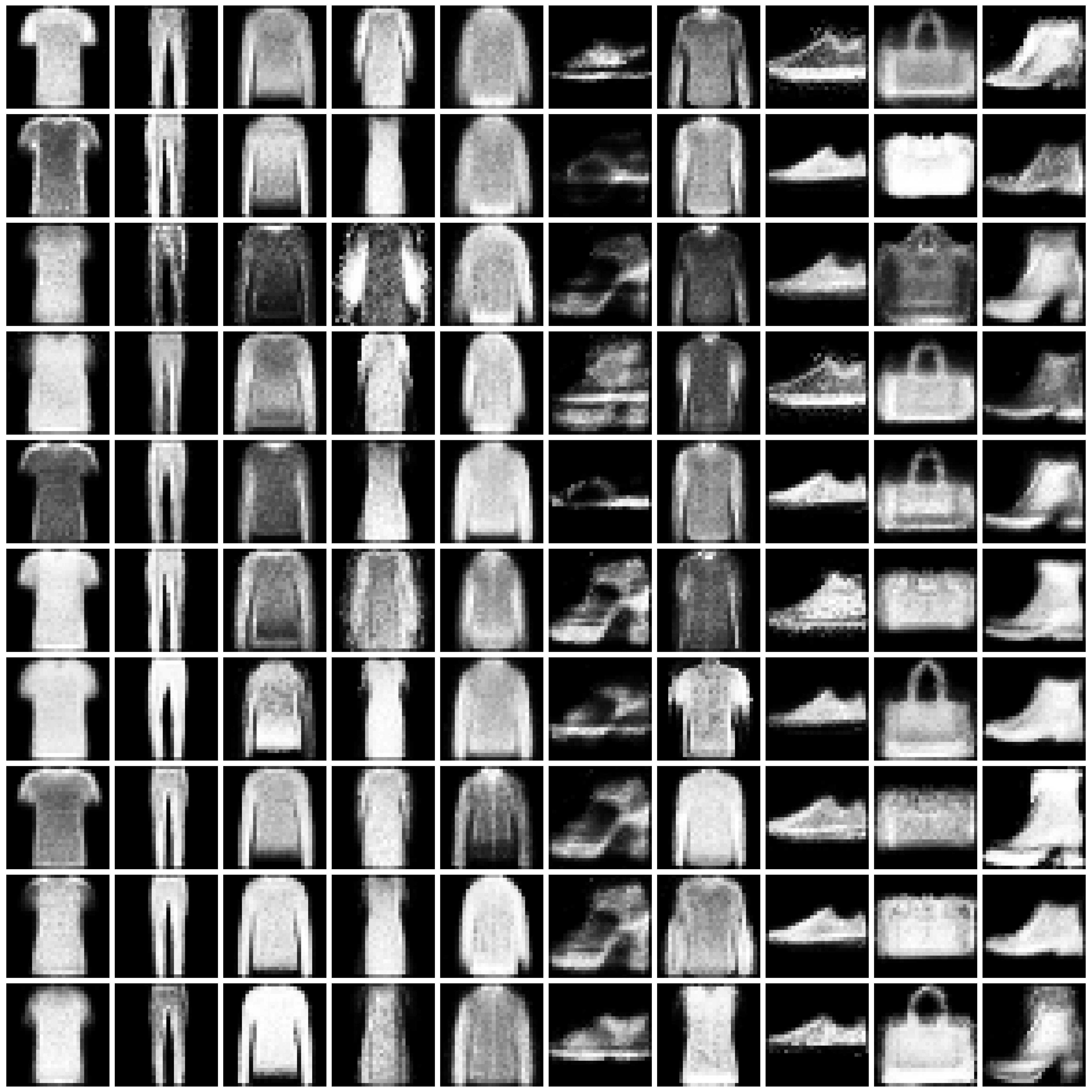
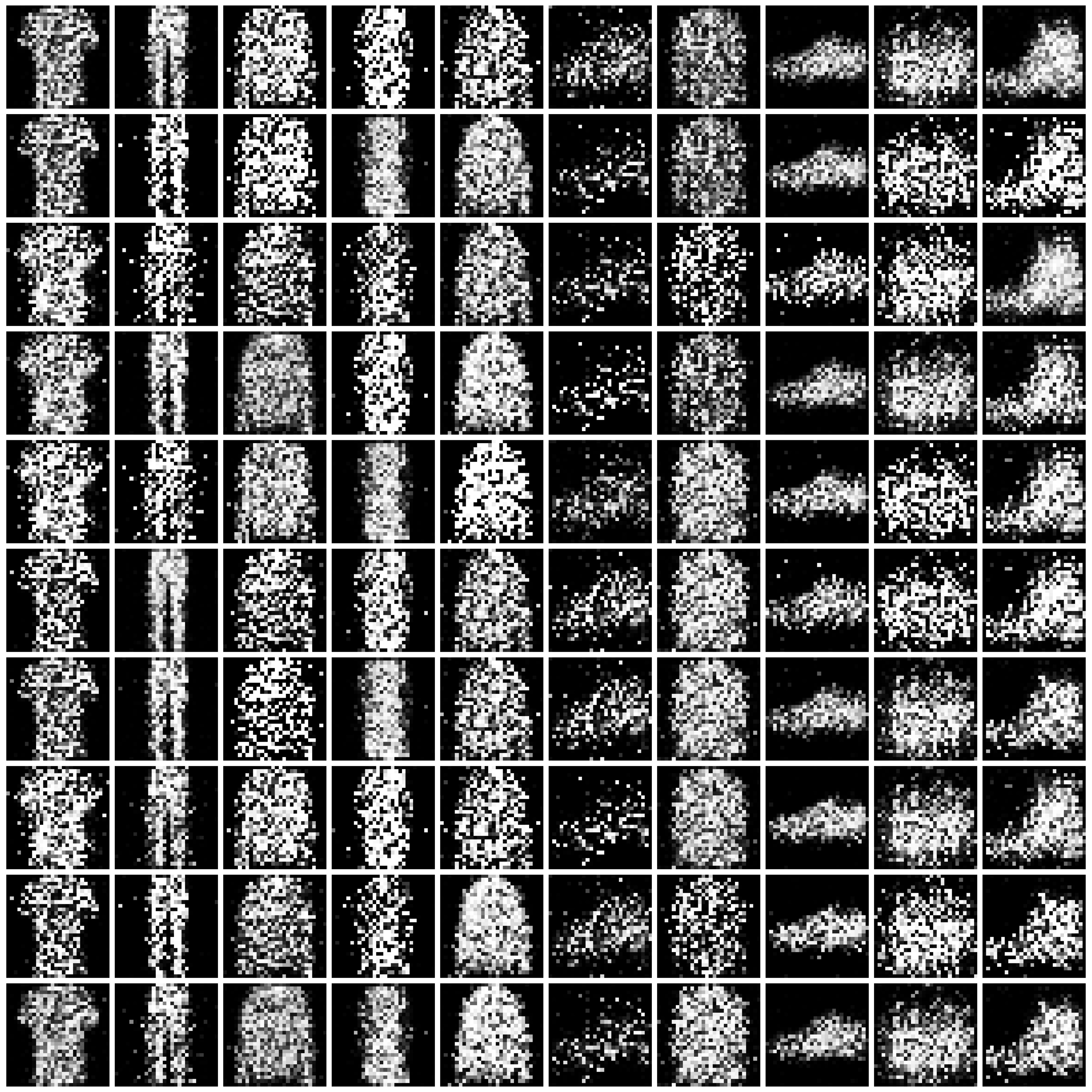
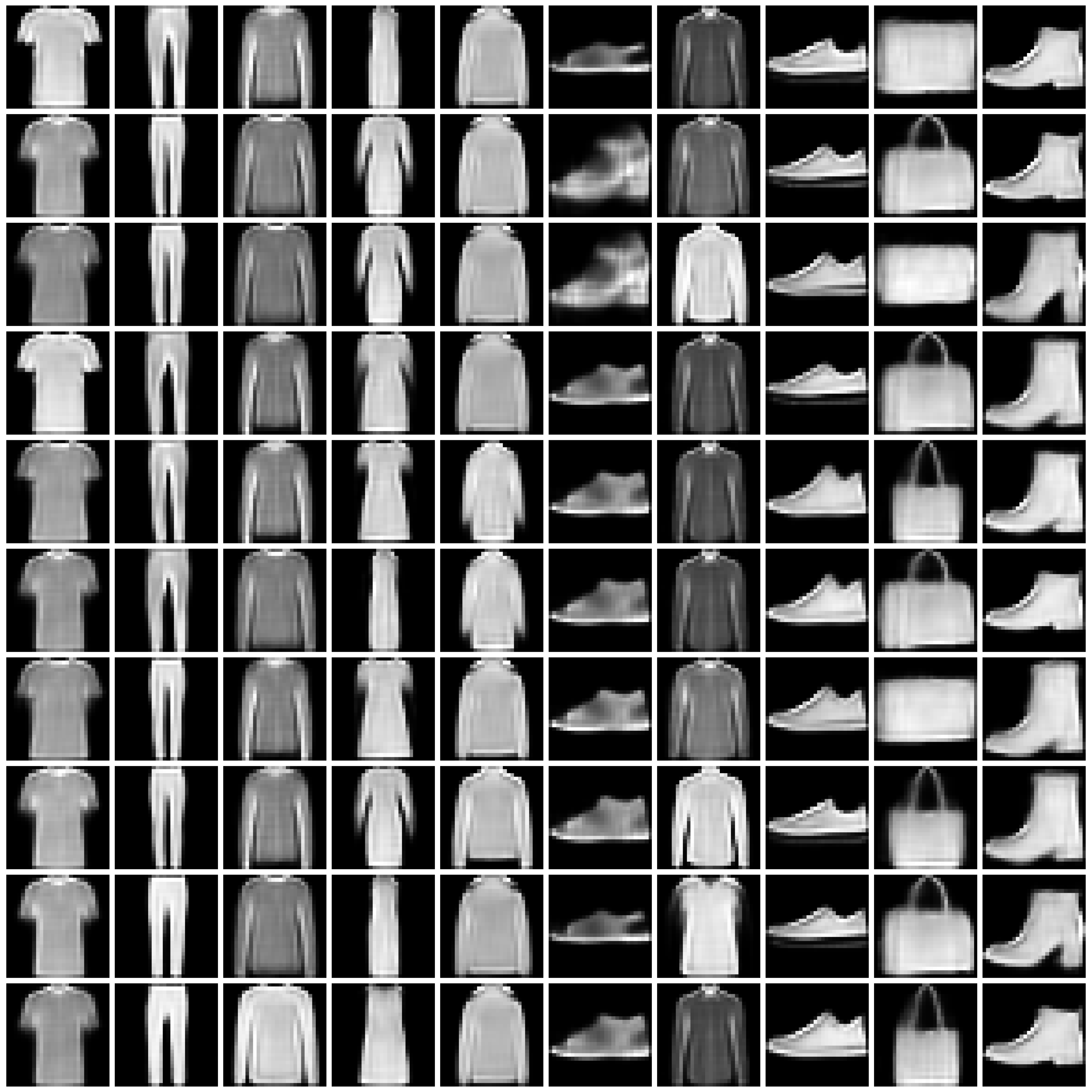
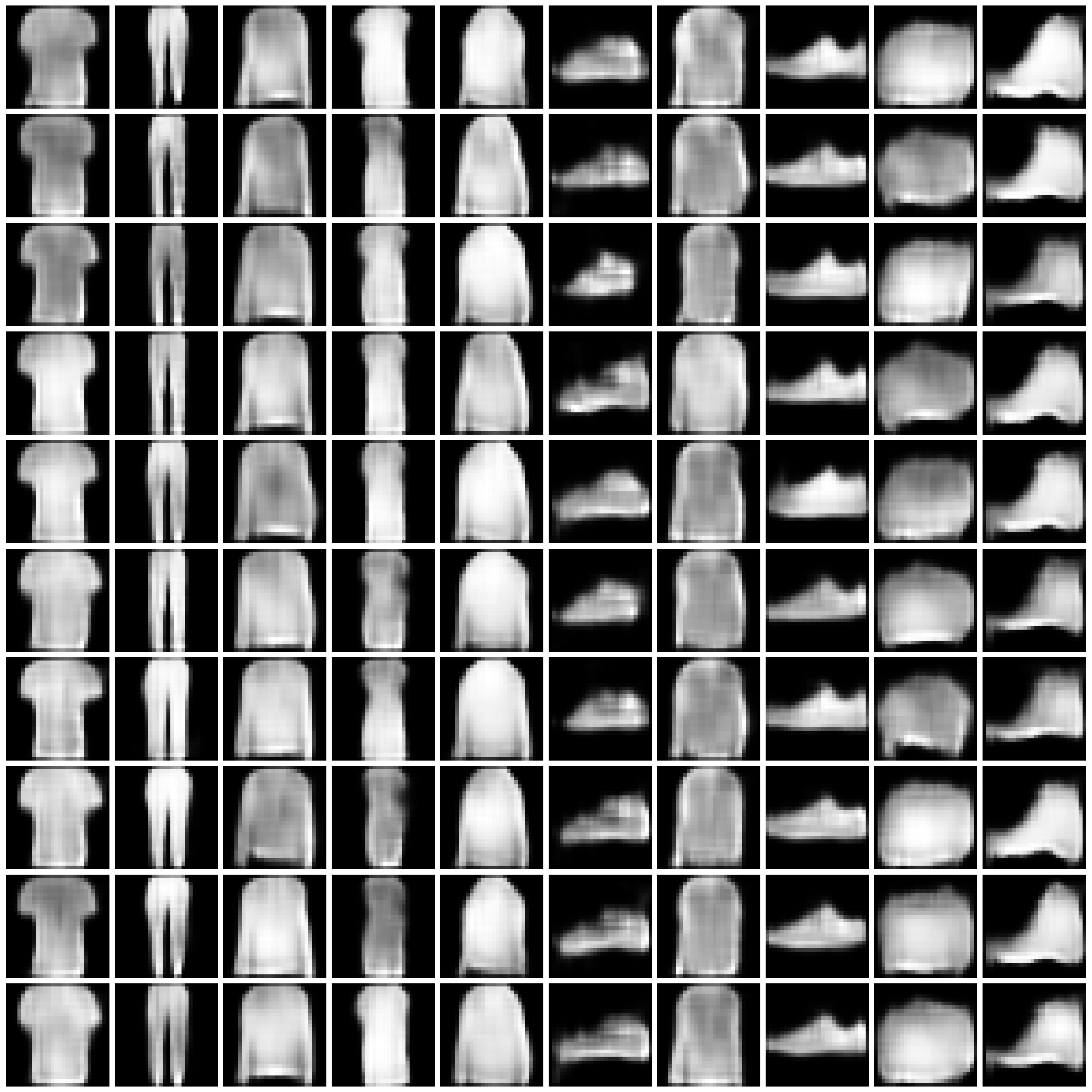
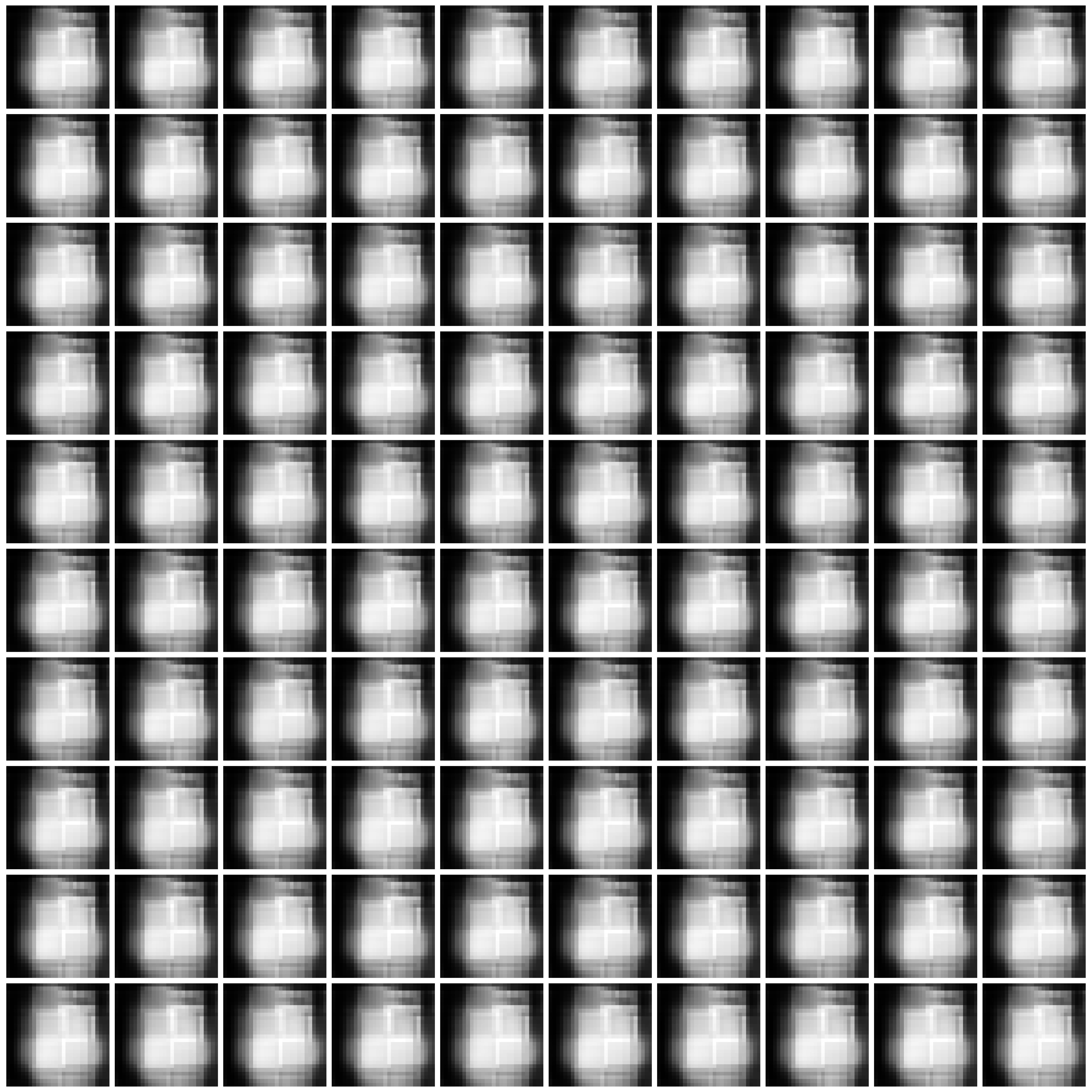
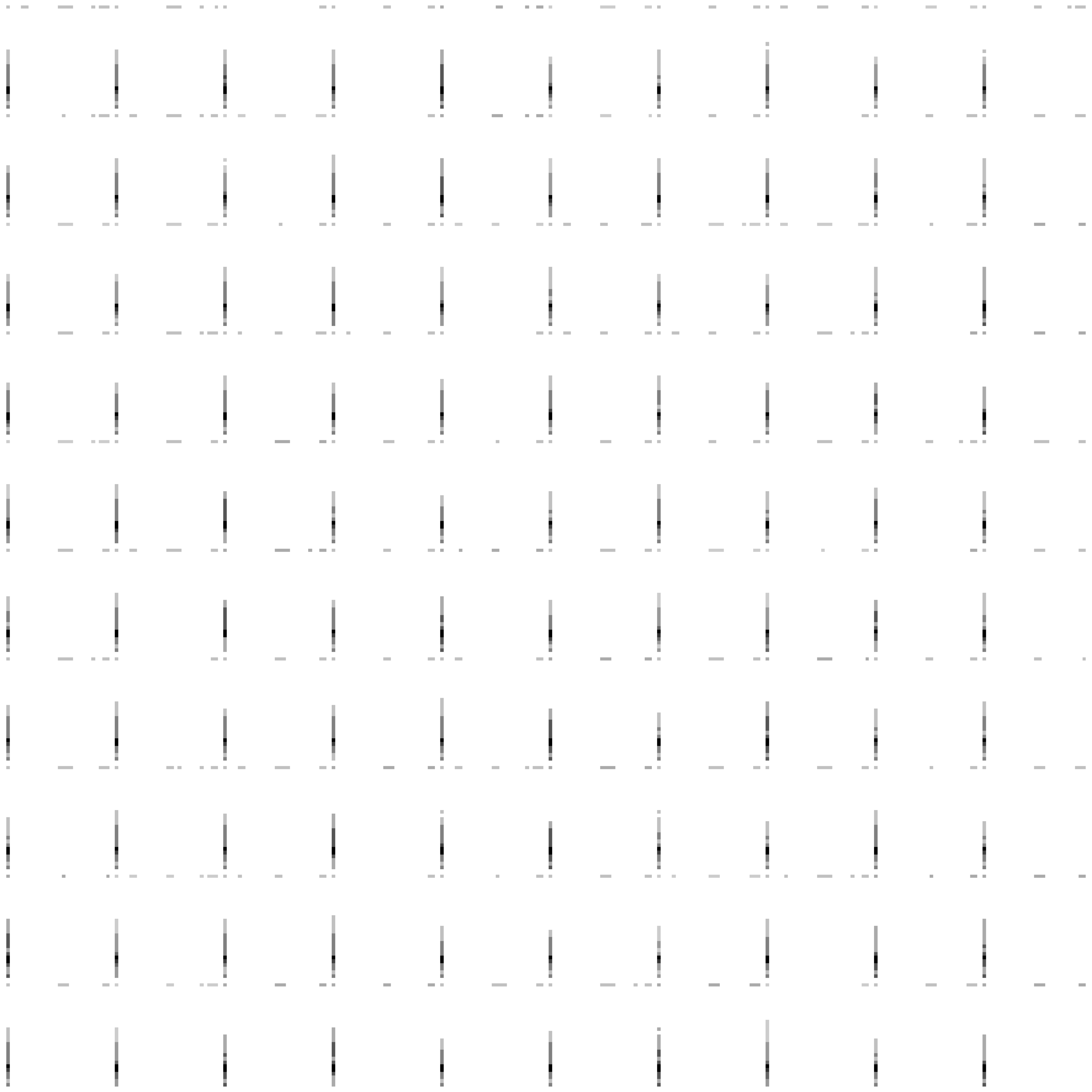
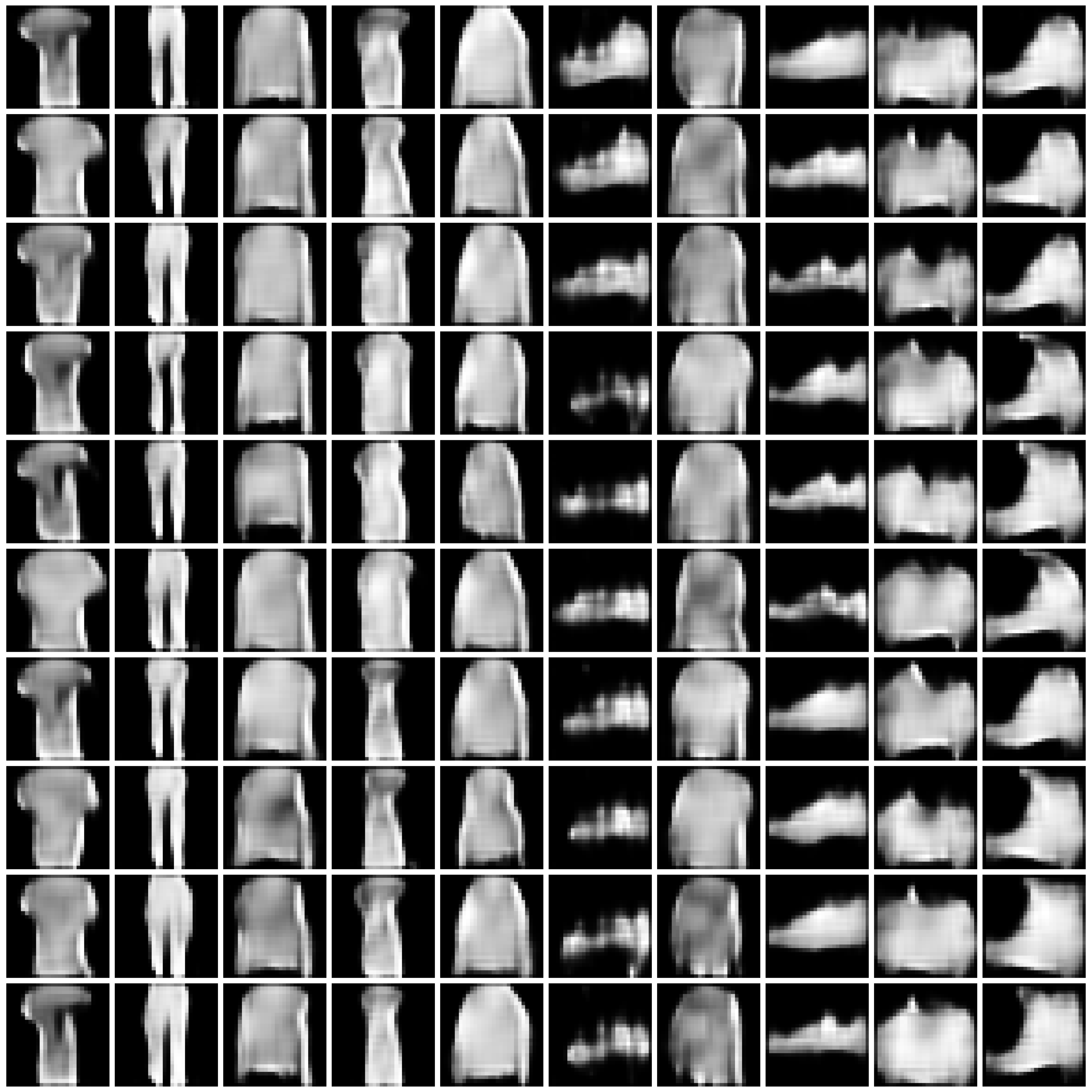
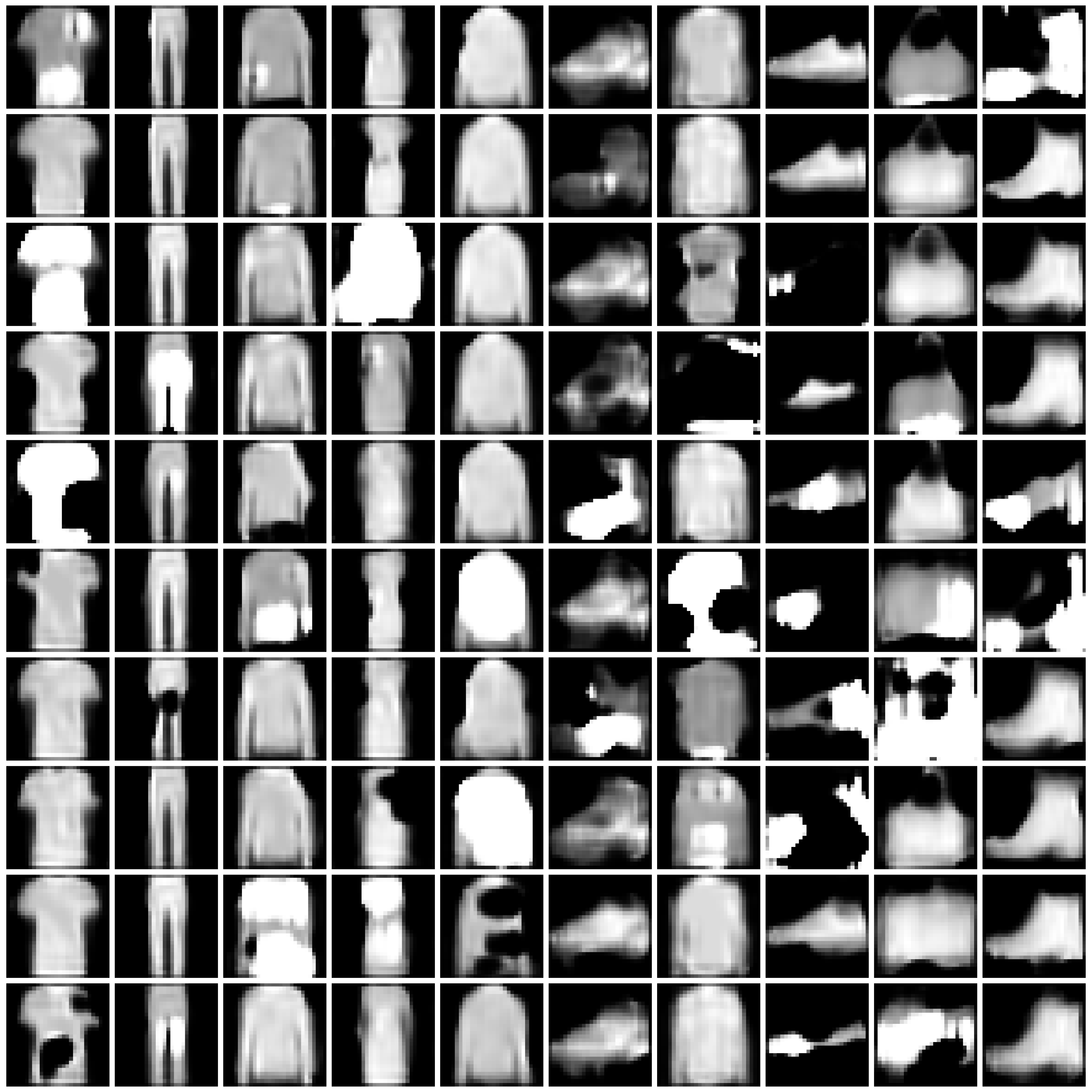
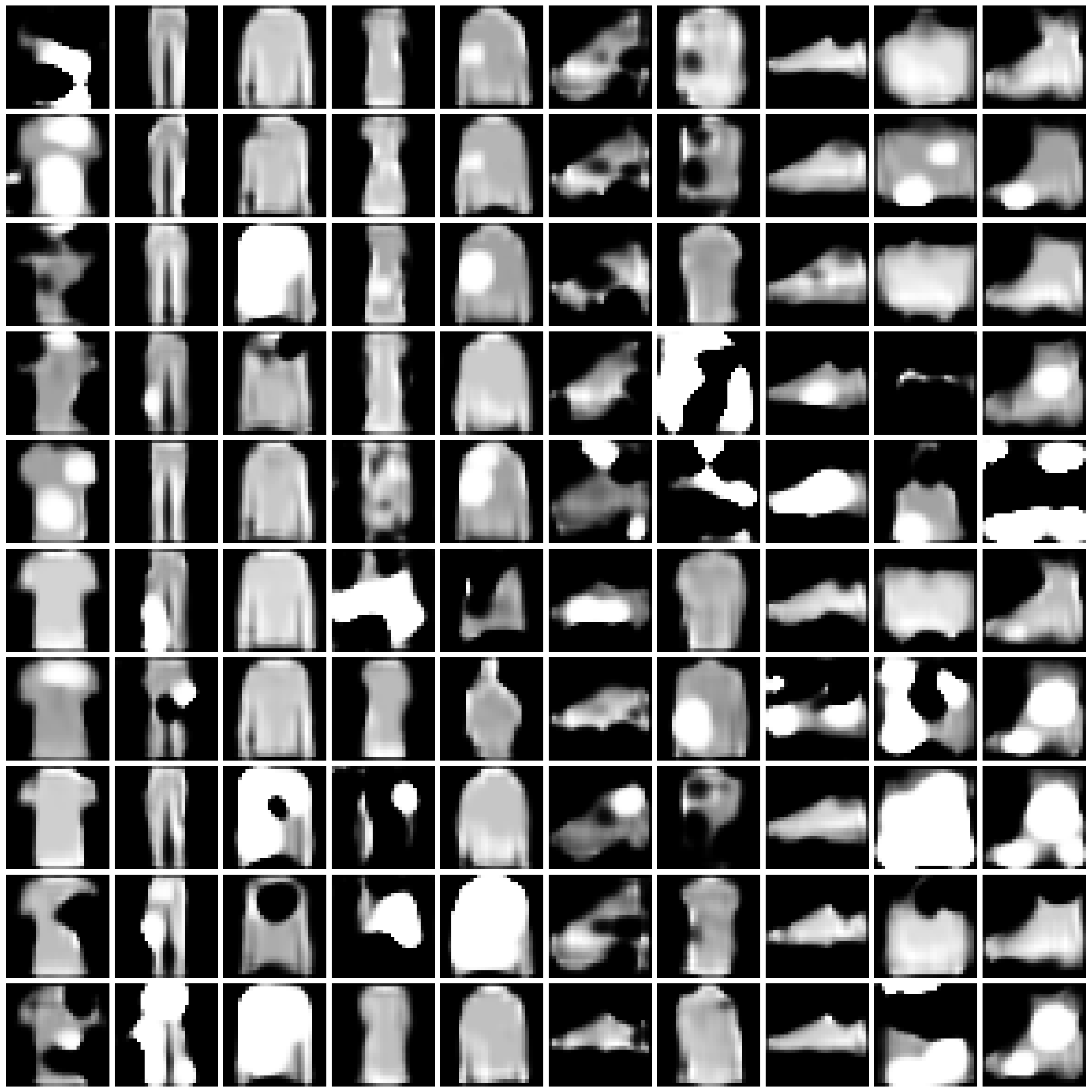
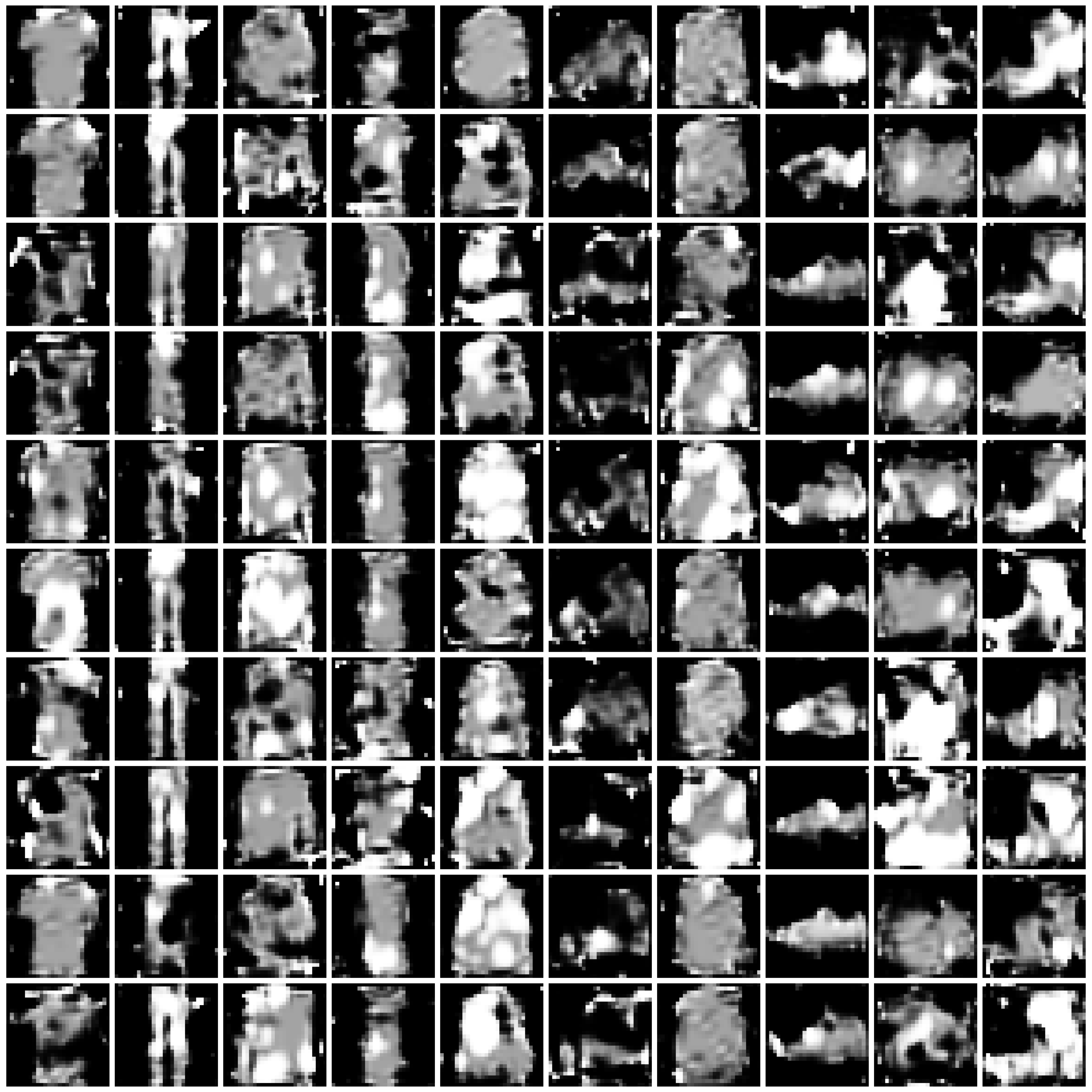
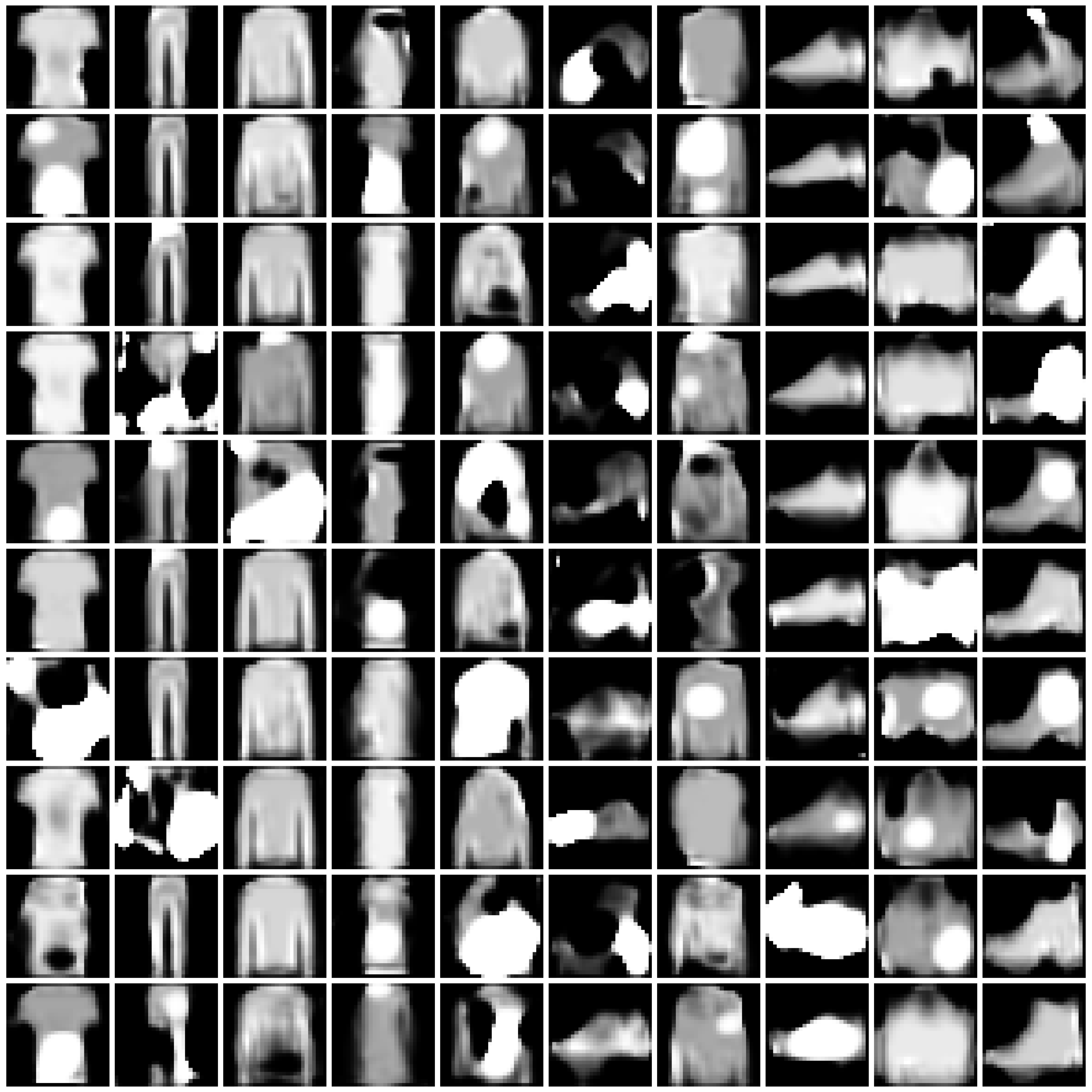
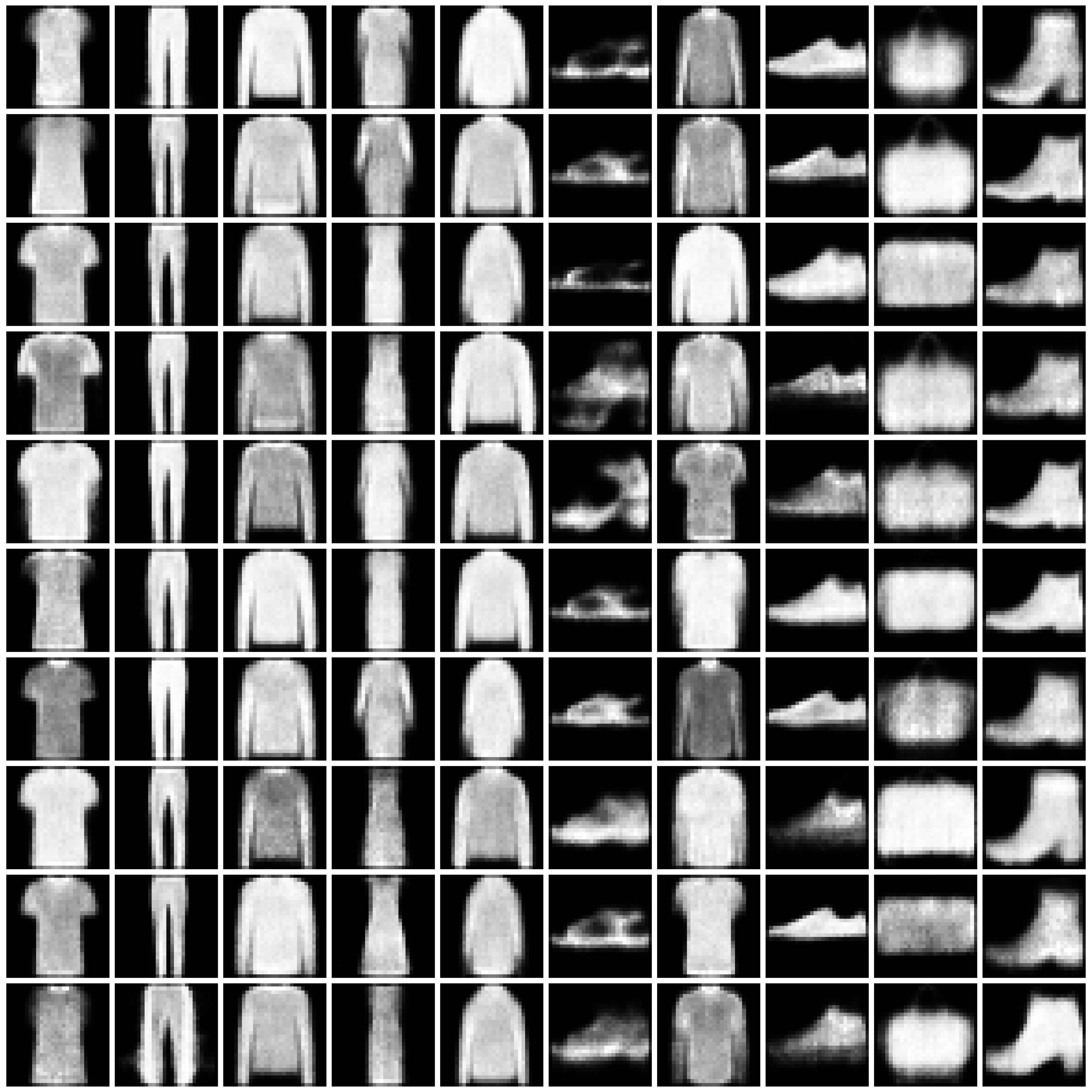
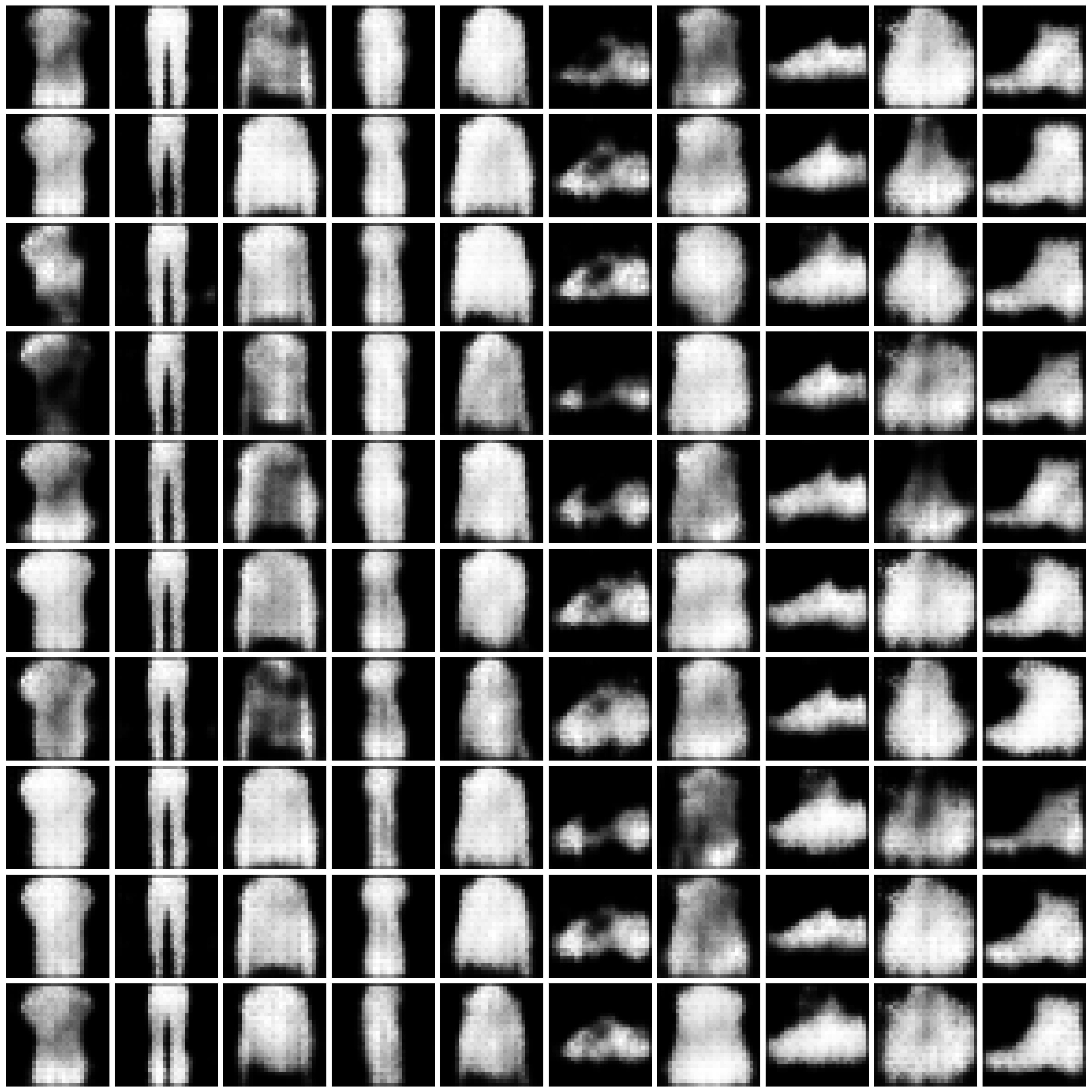
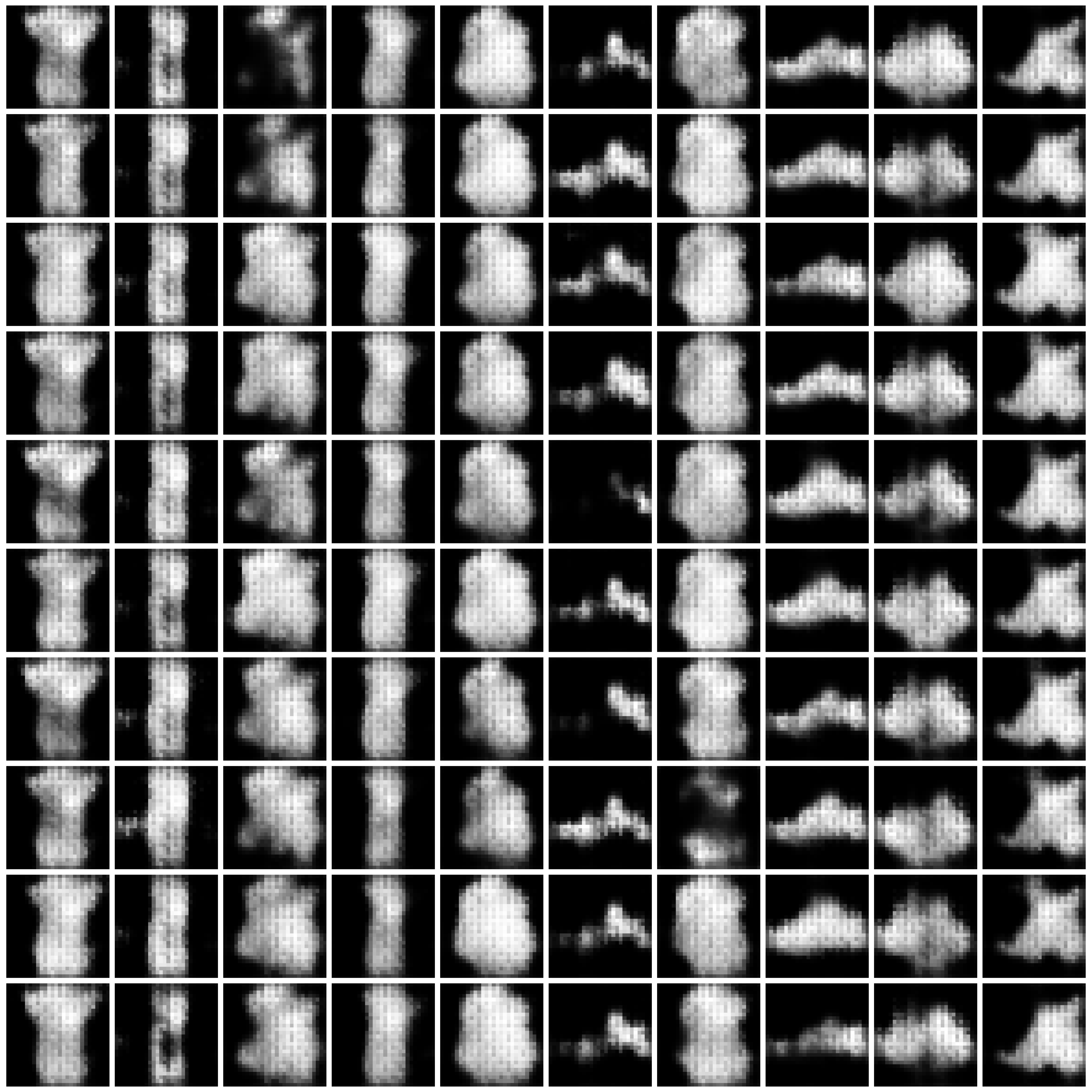
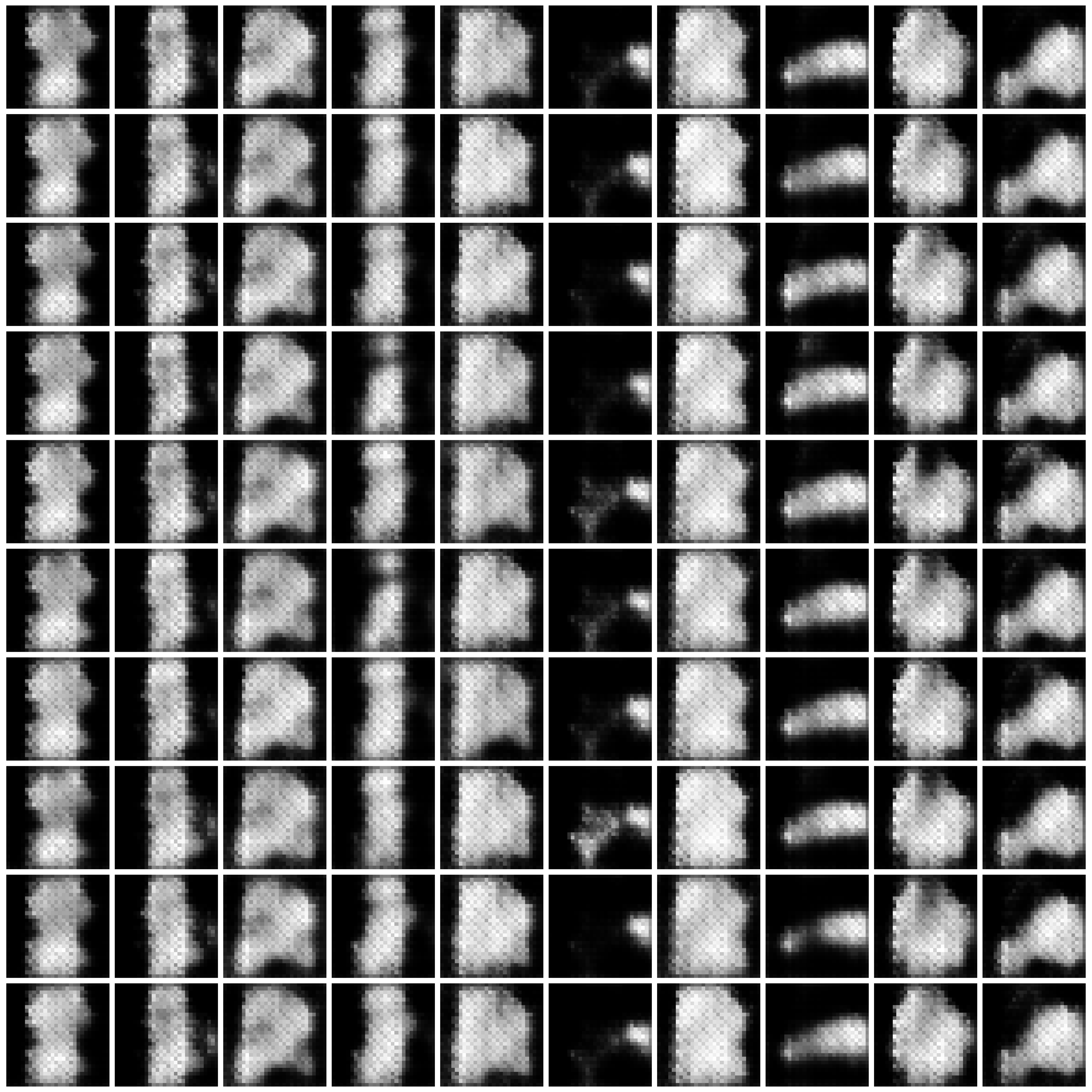
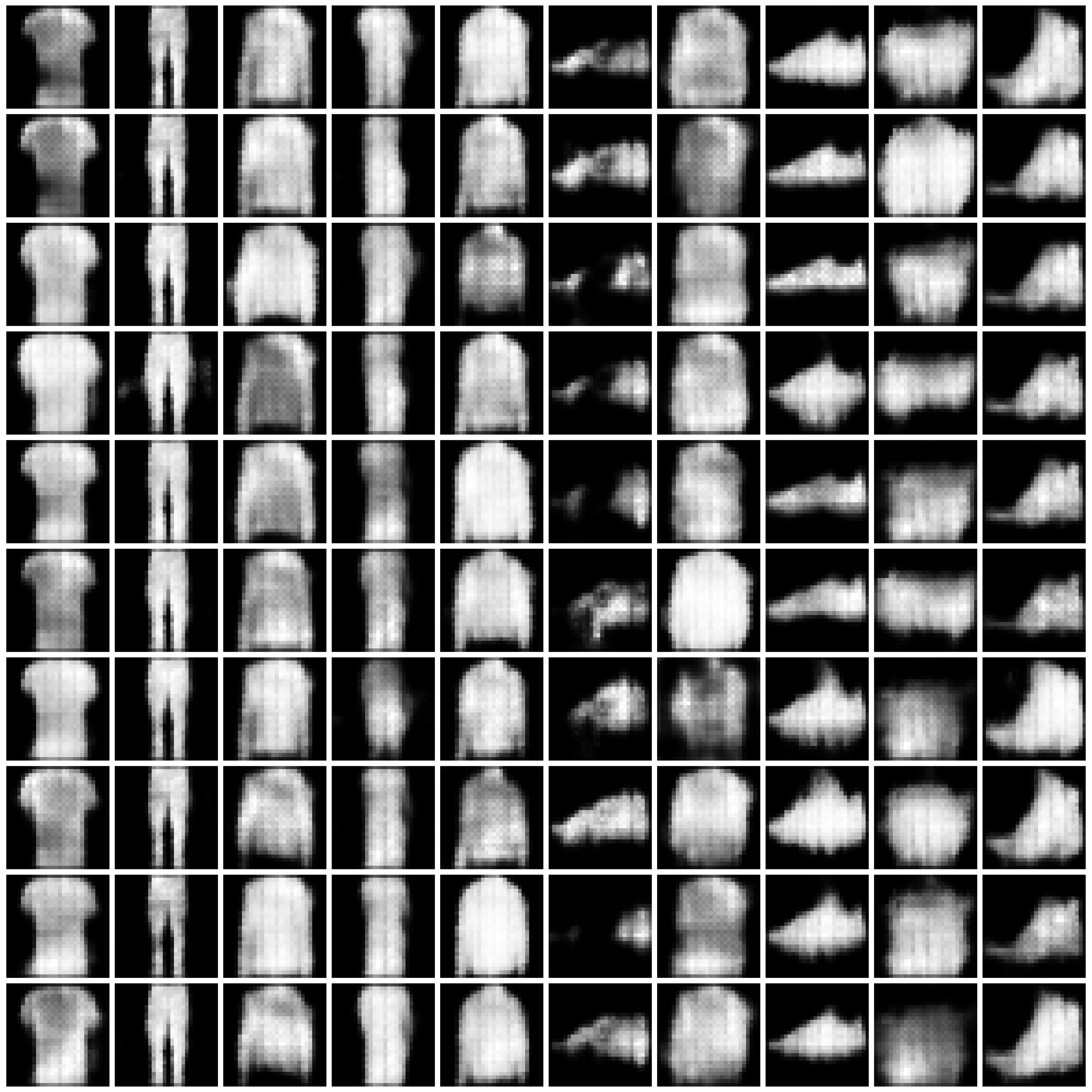
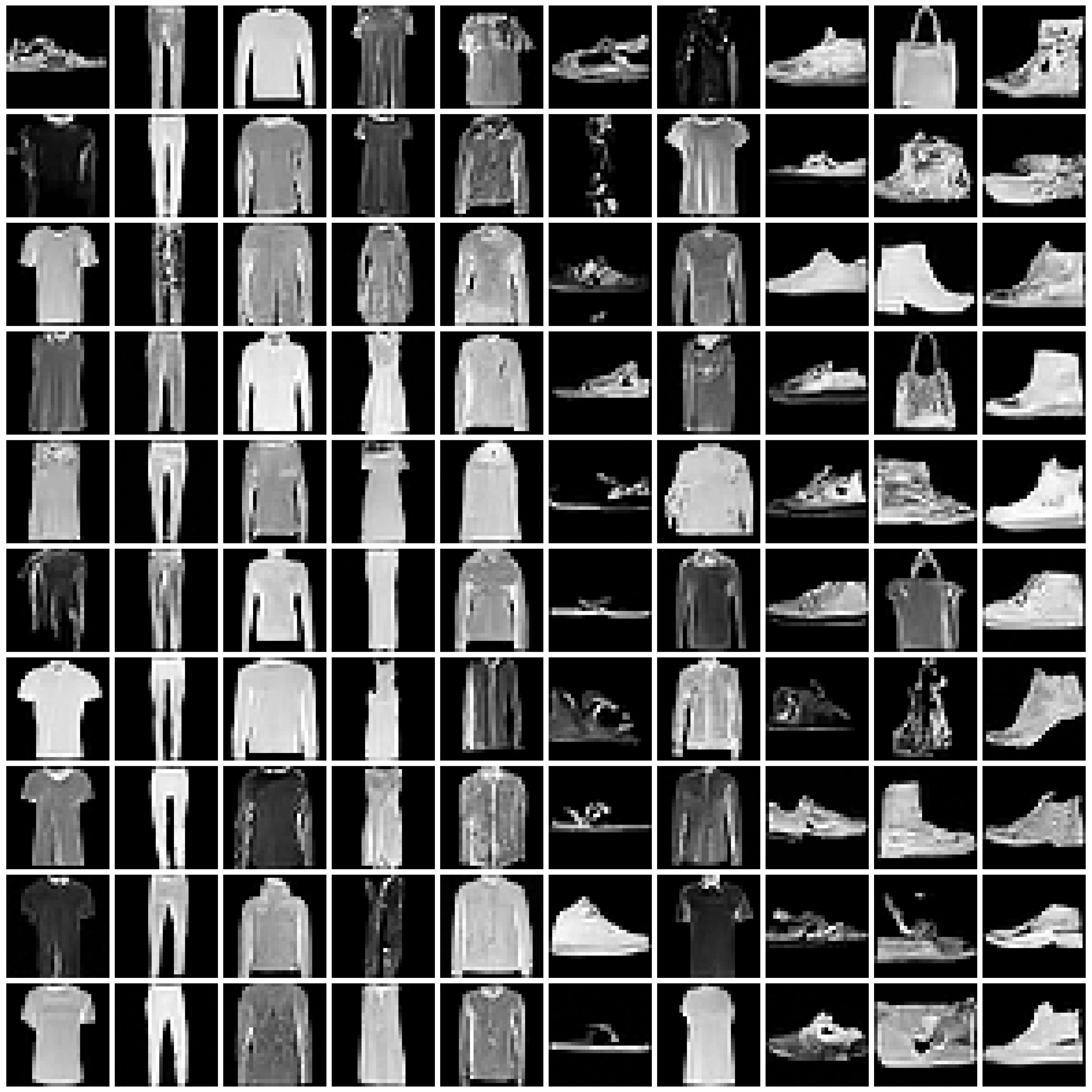
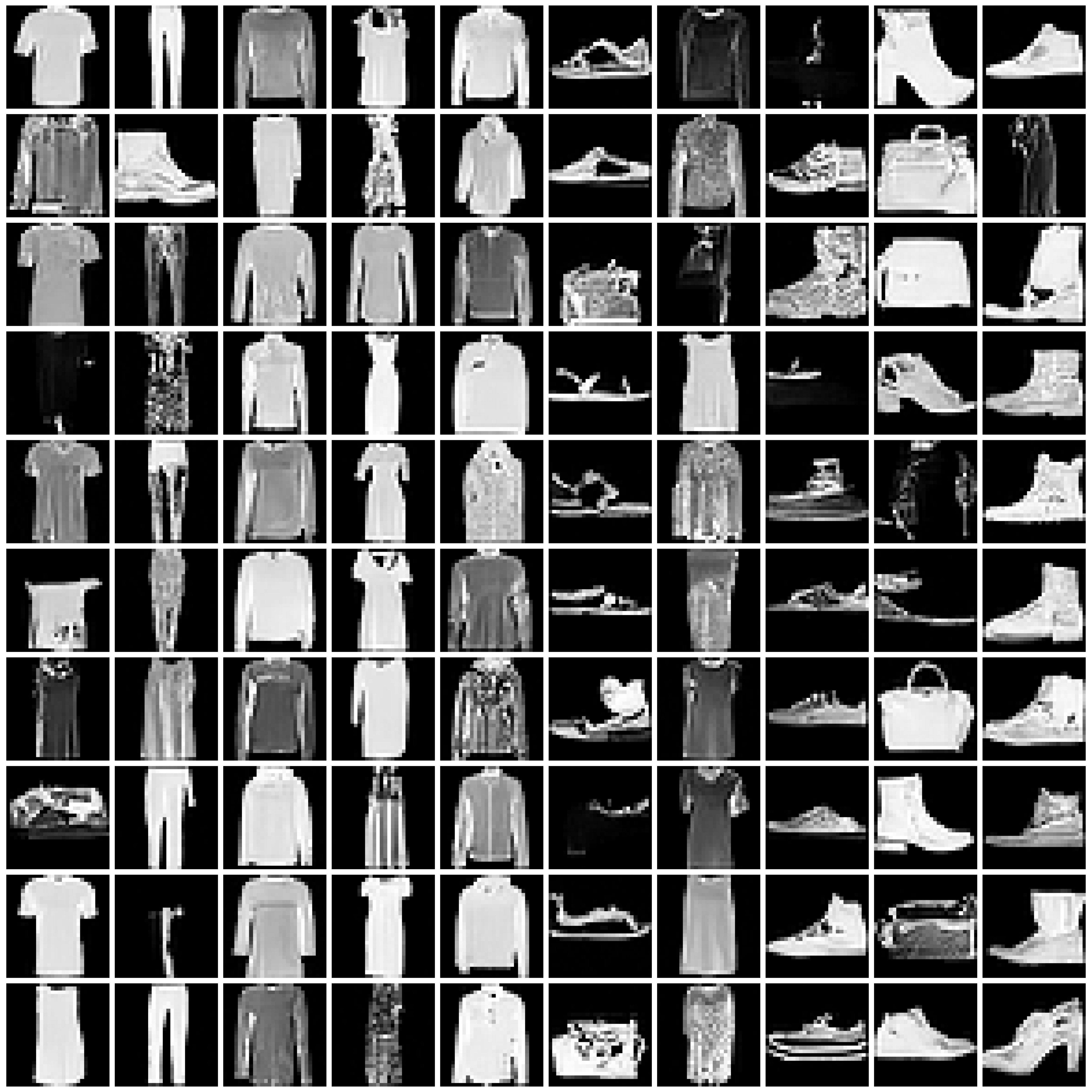
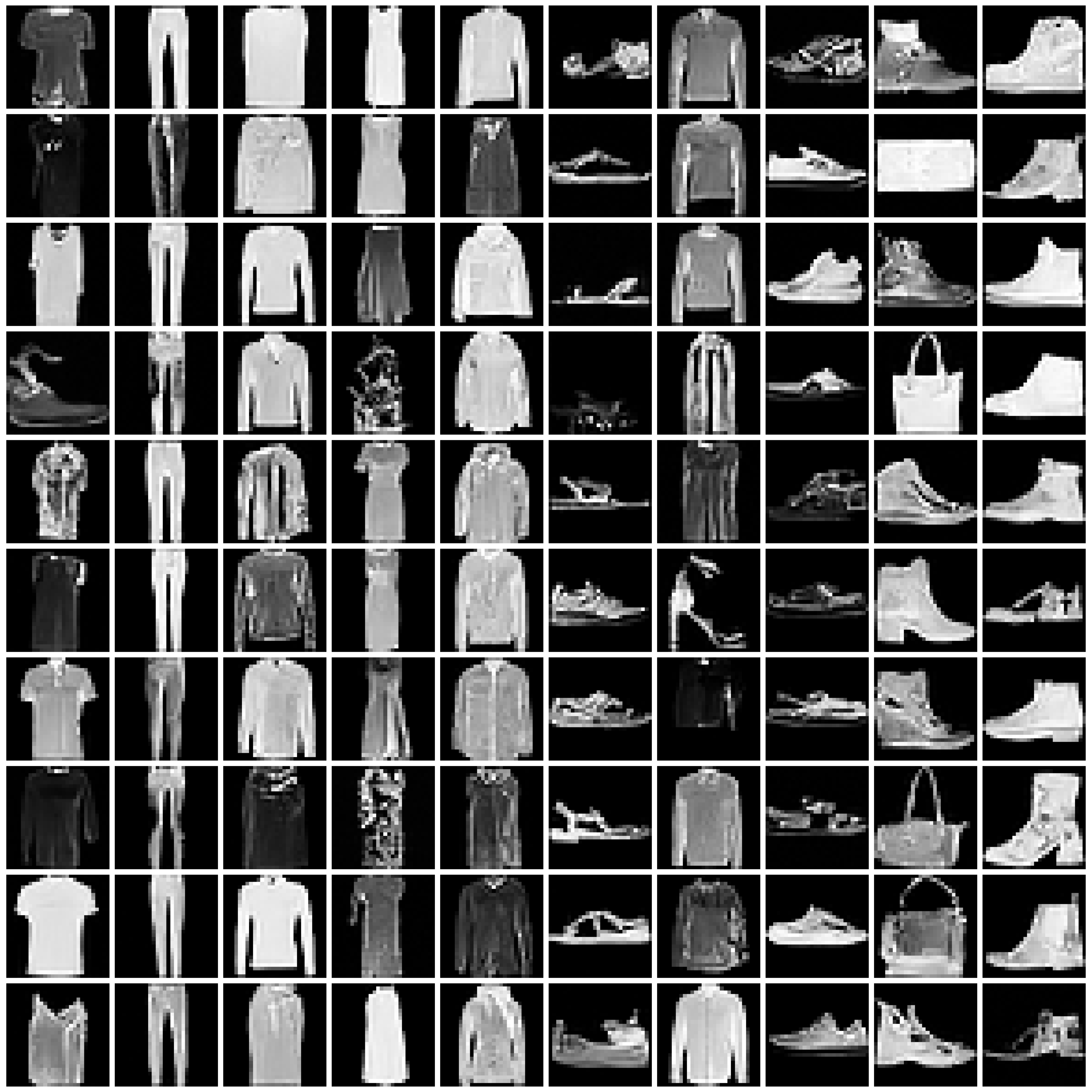
We present the synthesized images produced by each approach under each scenario.
For the combination of each approach and scenario, we randomly sample 10 images for each class. We present the images in 10x10 grids, where each column corresponds to one class.
Refer to Fig. 1 and Fig. 2 for the images synthesized by different approaches on MNIST and Fashion-MNIST.
Note to readers:
-
The images are big; please allow some time for them to load.
-
To have a clearer view, you can right click the image and choose “Open Image in New Tab”.
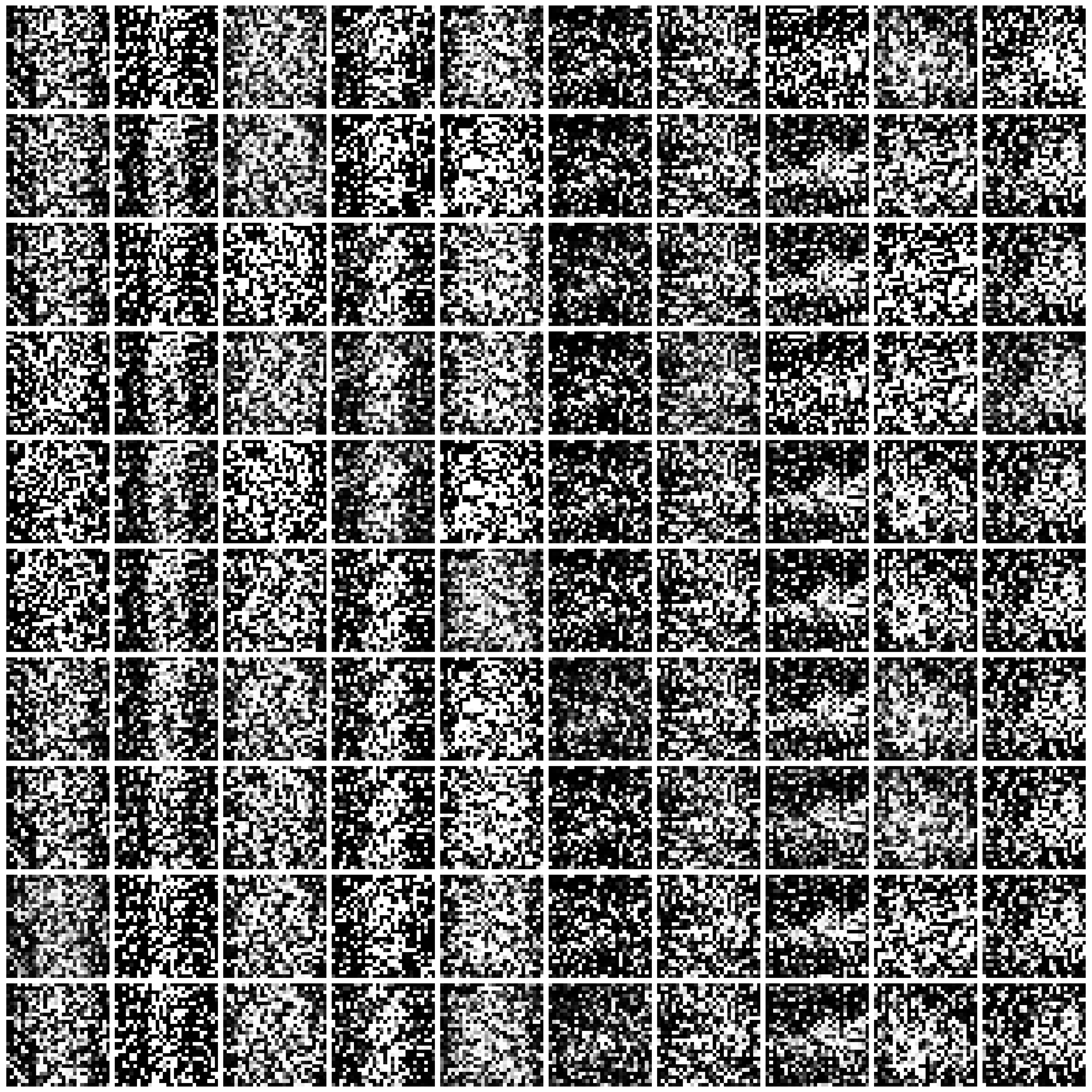
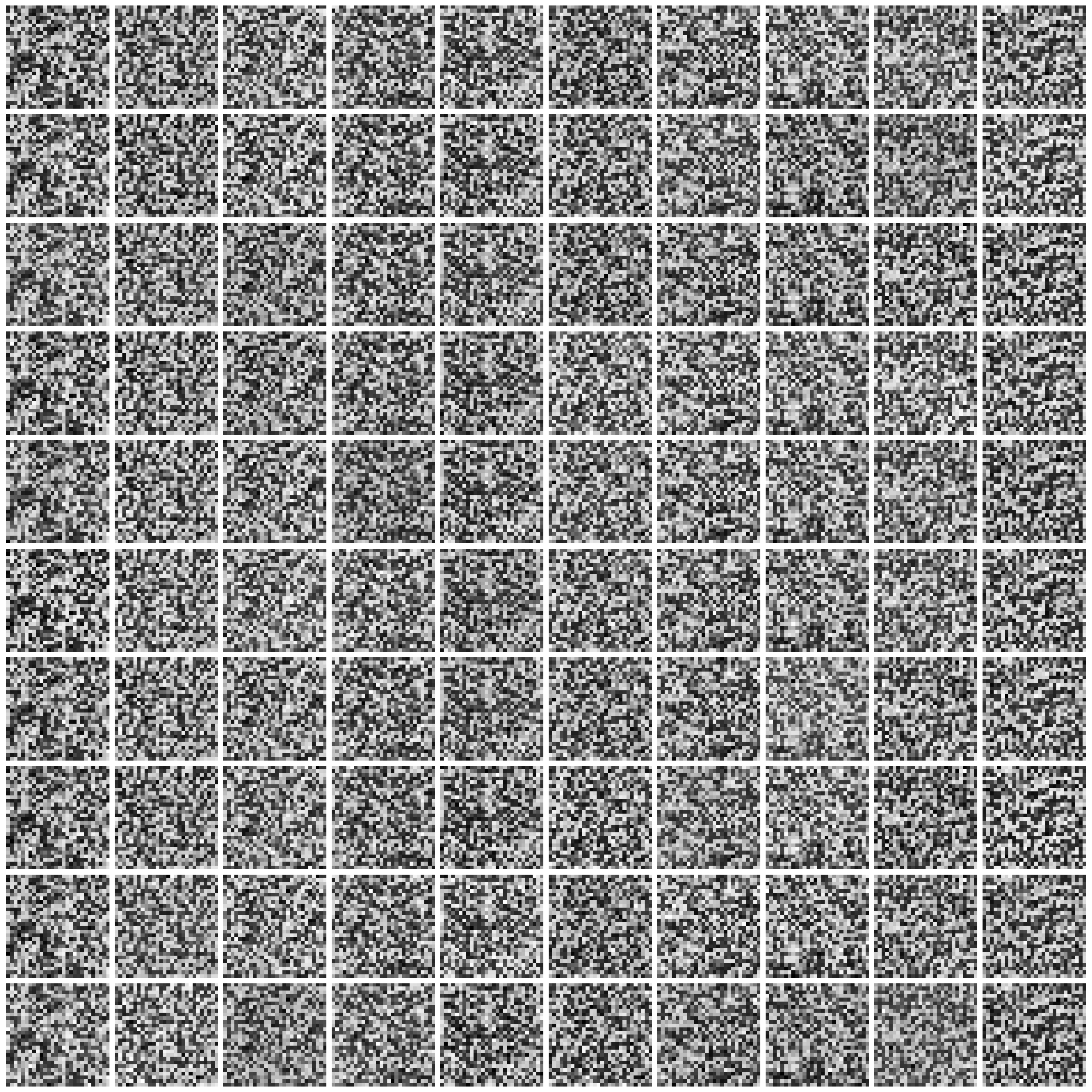
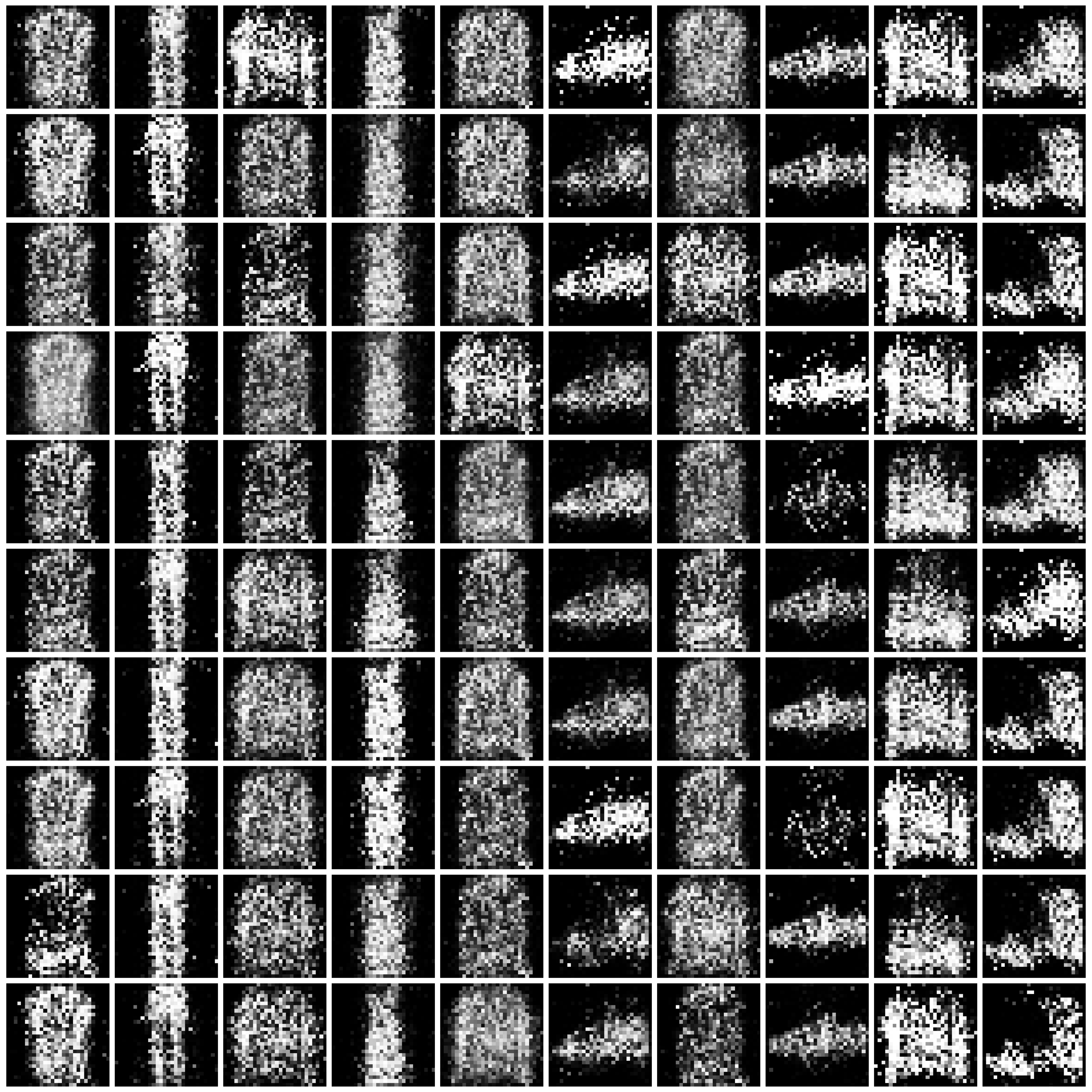
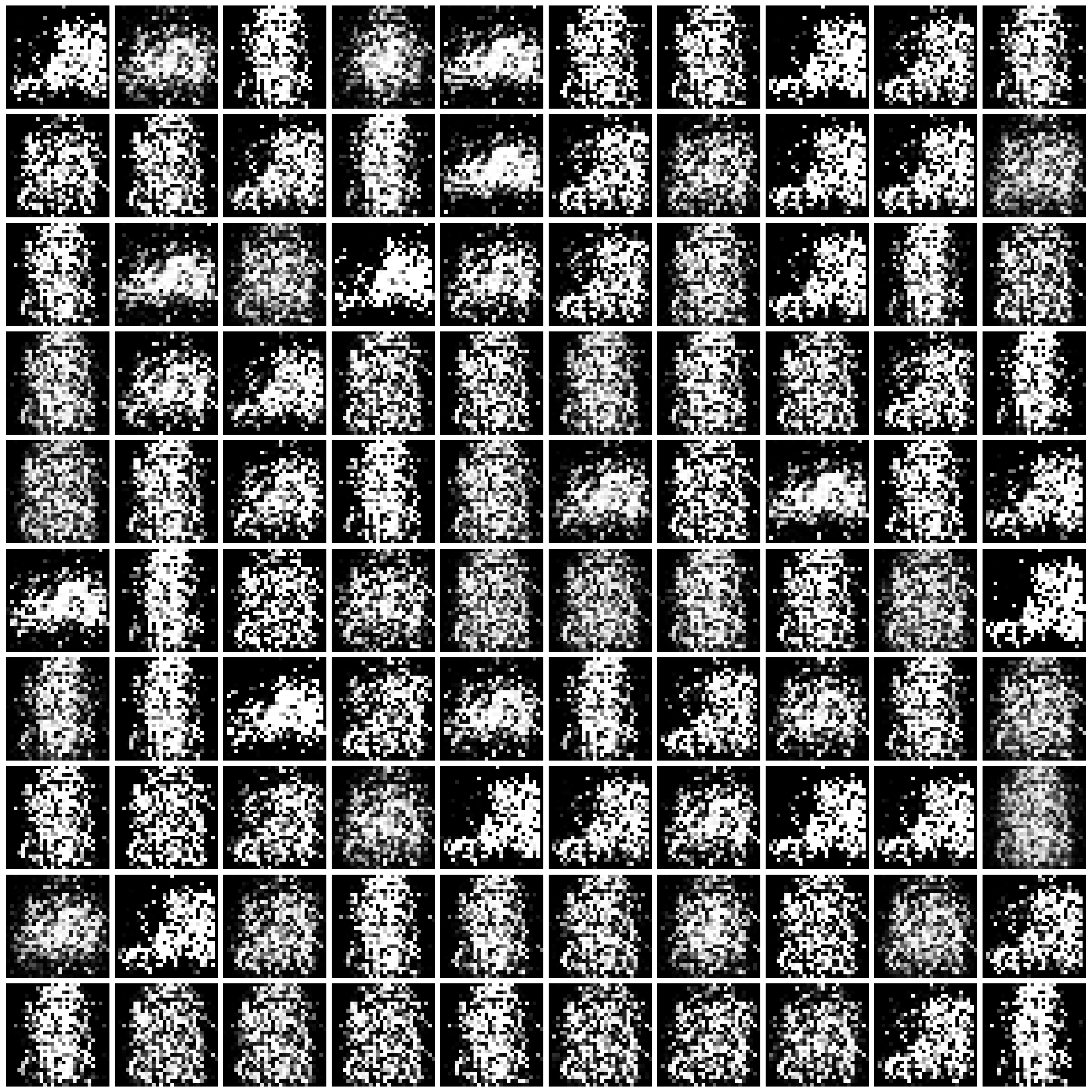
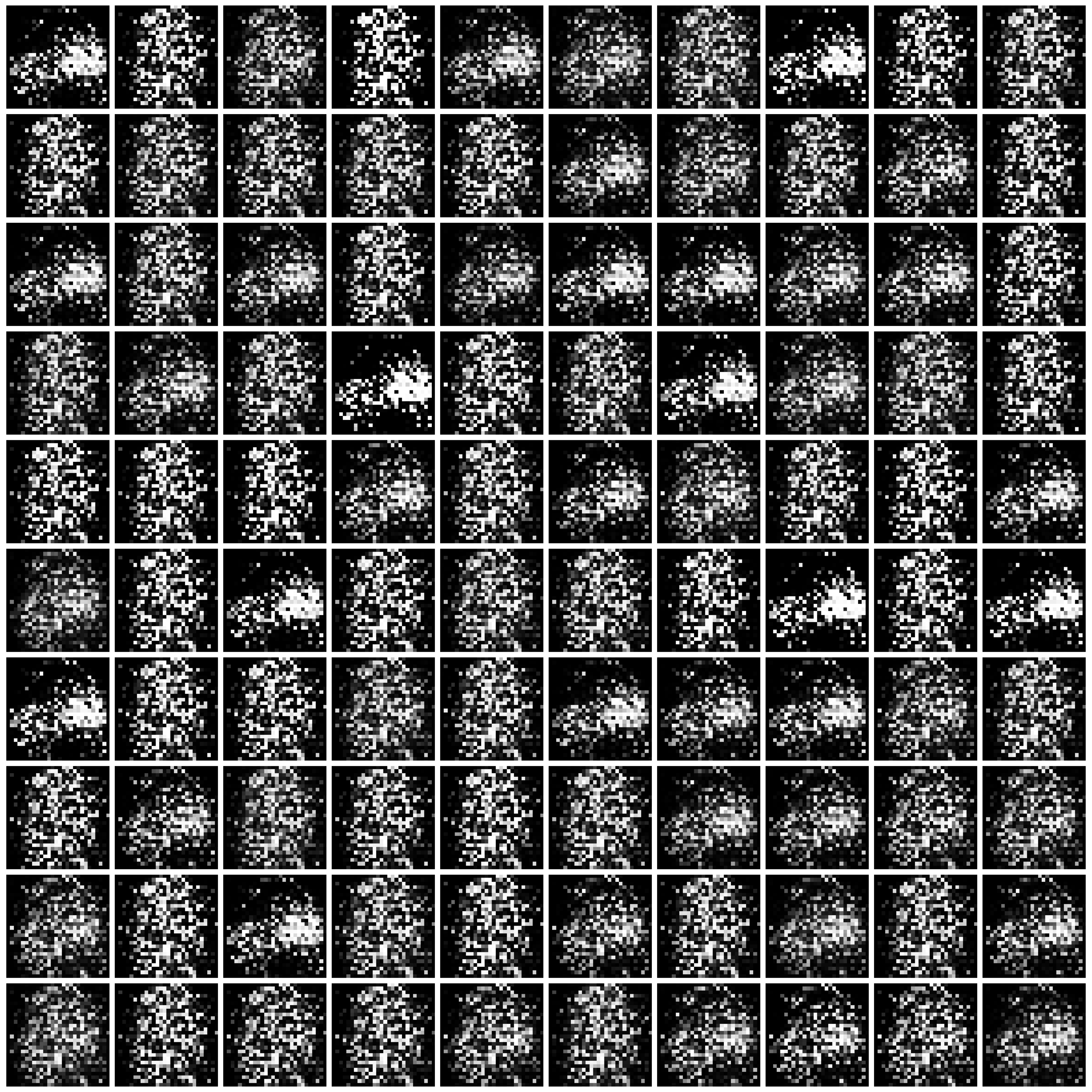
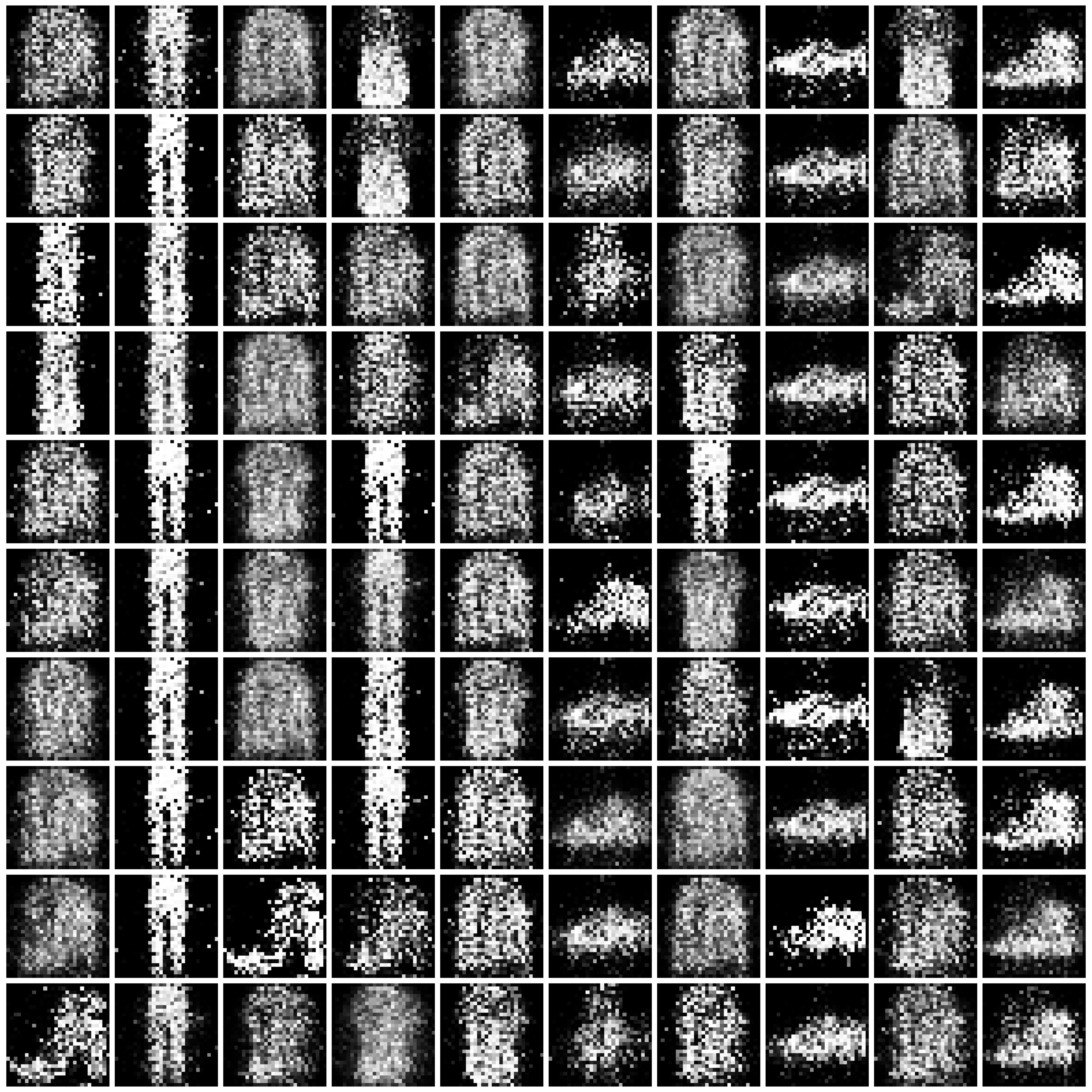
Figure 1: Synthesized Images by different approaches on MNIST dataset. The five columns are “non-private”, “$\varepsilon=10$”, “$\varepsilon=1$”, “$\varepsilon=0.2$”, and “half” from left to right.
| DPGAN |
|
|
|
|
|
| DP-CGAN |
|
|
|
|
|
| GS-WGAN |
|
|
|
|
|
| DP-MERF |
|
|
|
|
|
| DP-Sinkhorn |
|
|
|
|
|
| DPGEN |
|
|
|
|
|
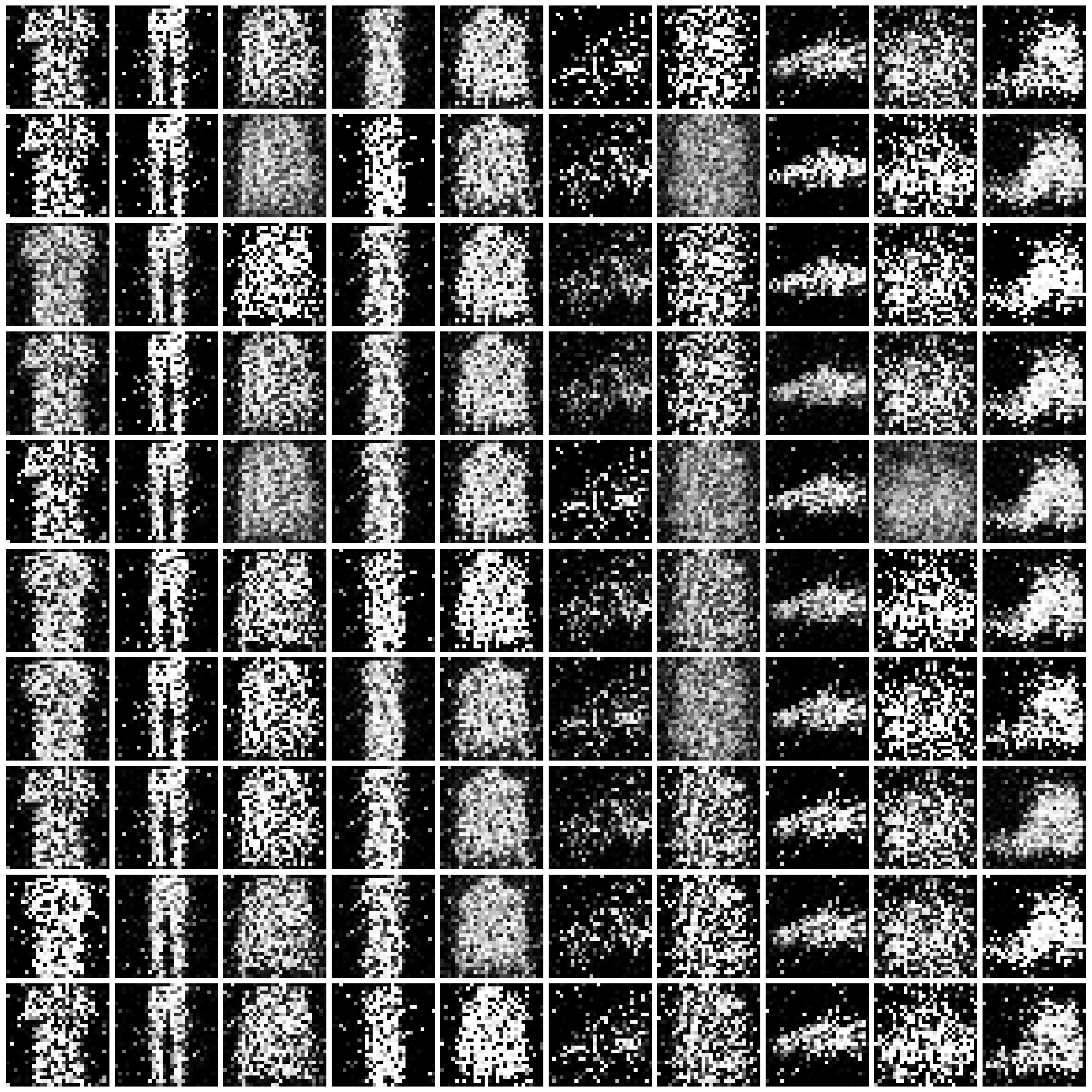
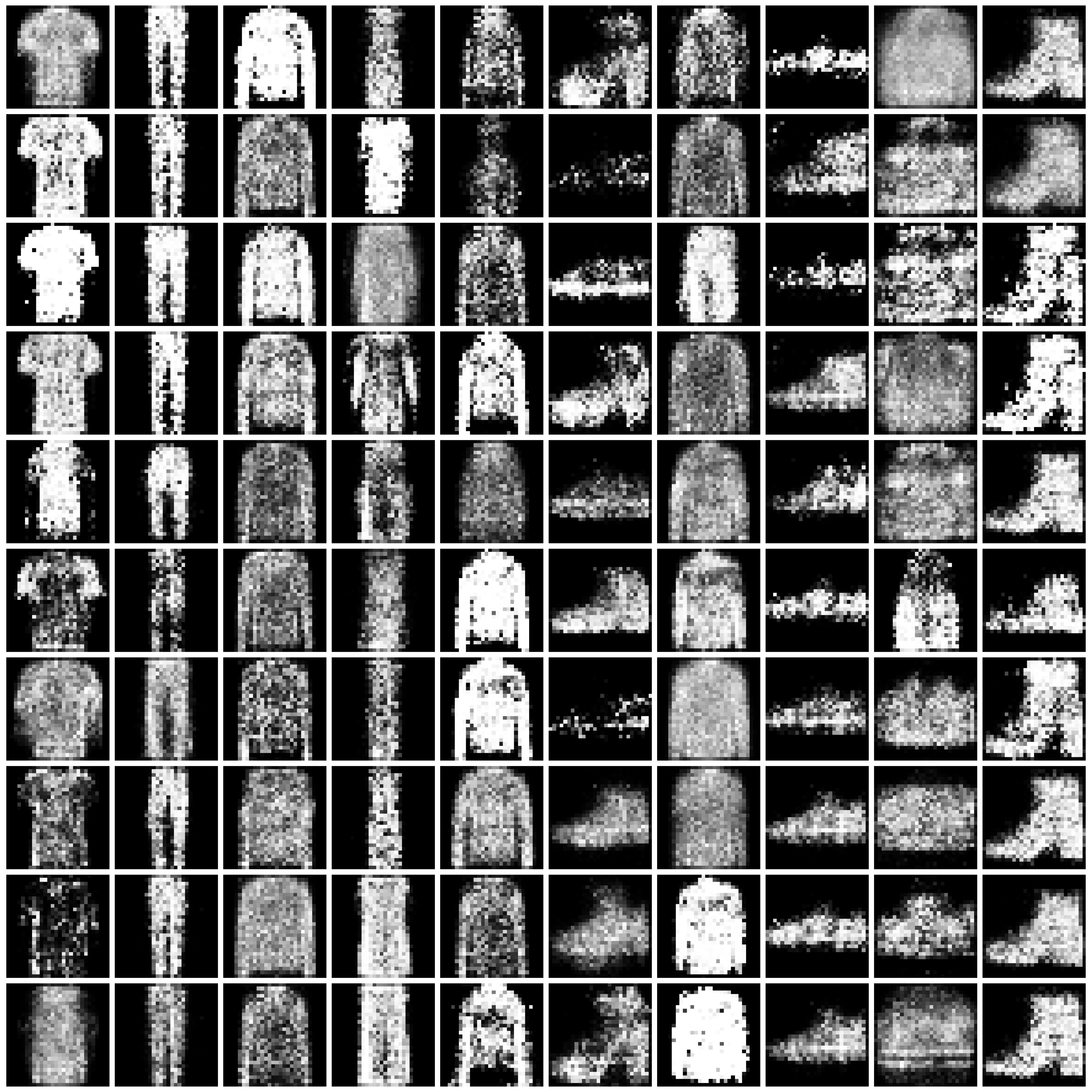
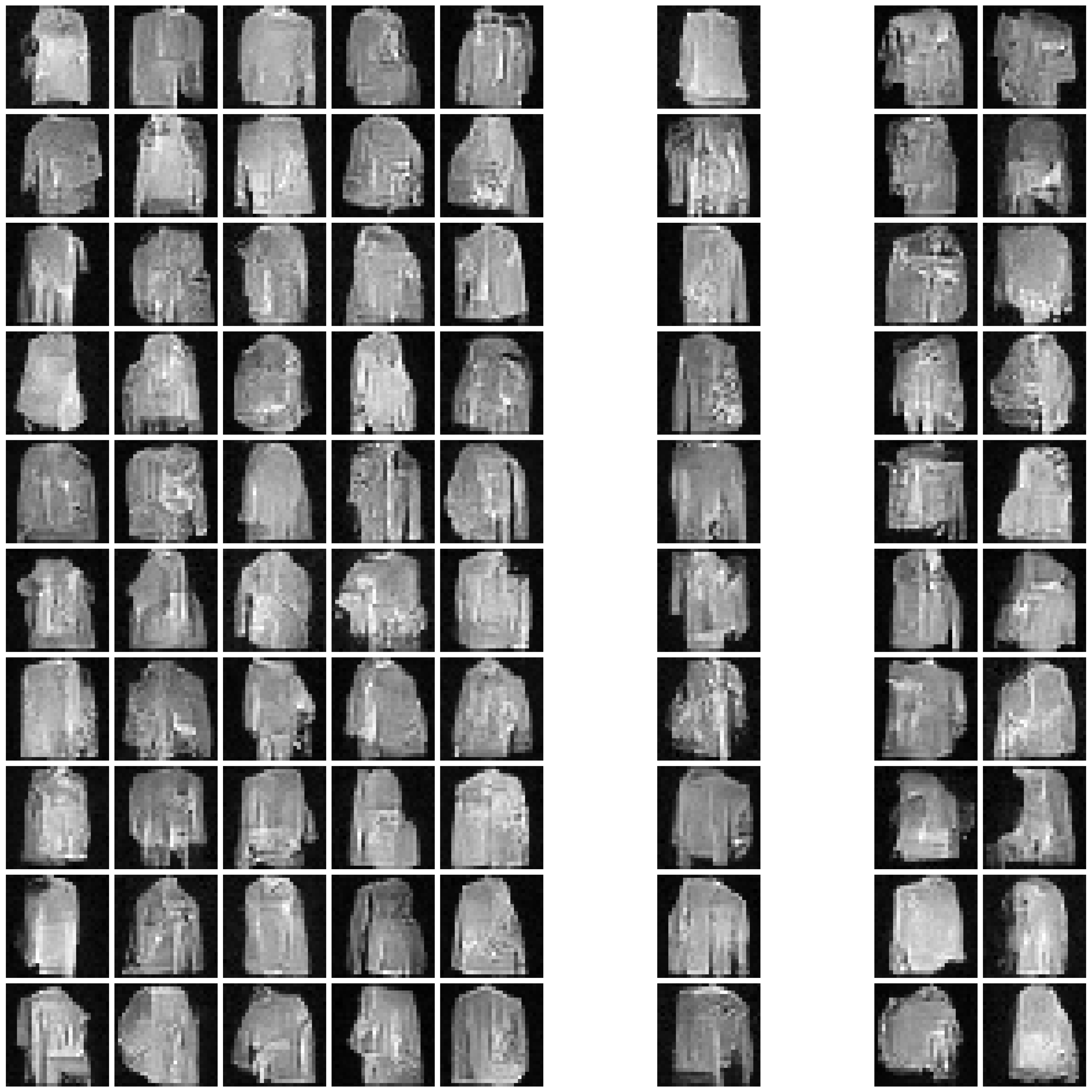
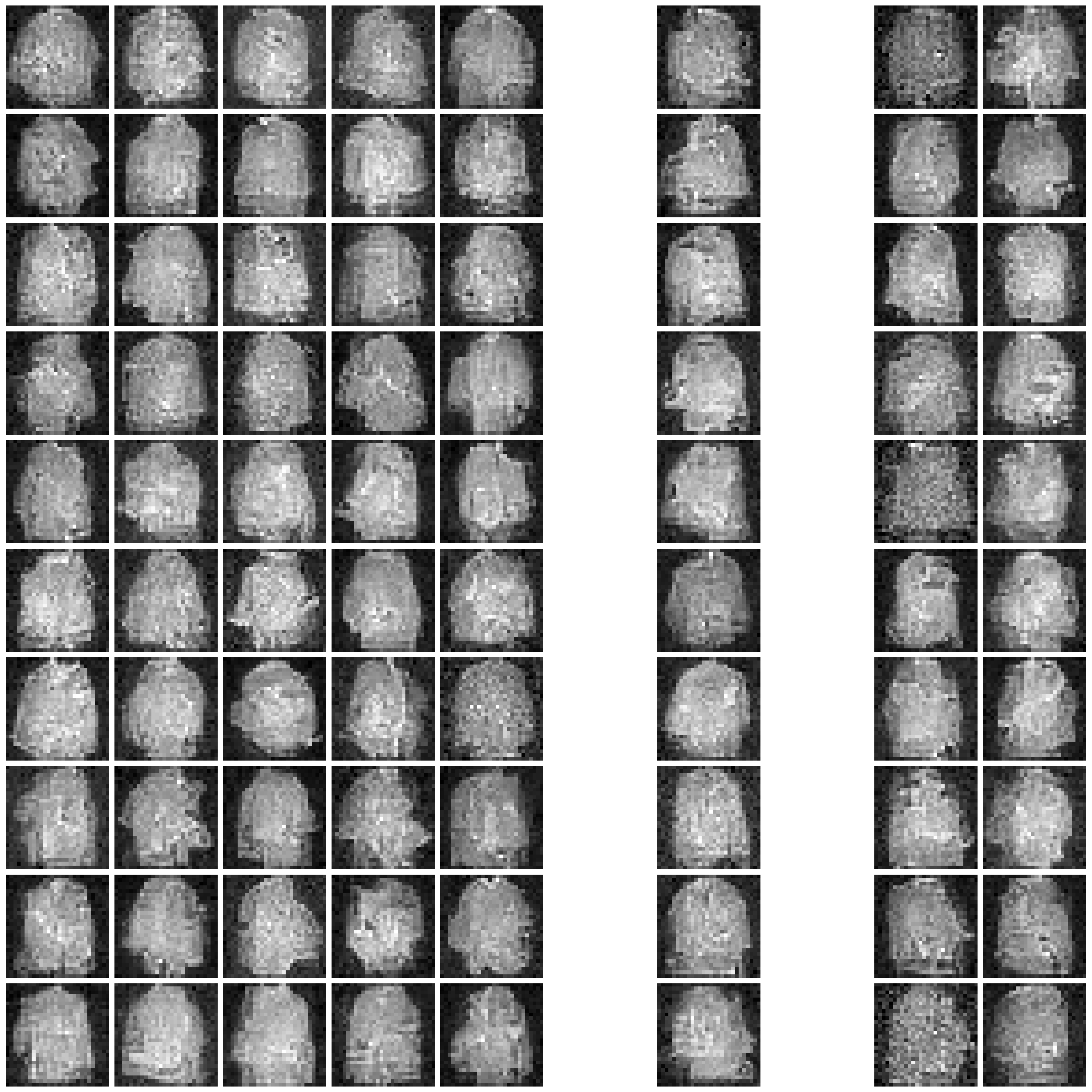
Figure 2: Synthesized Images by different approaches on Fashion-MNIST dataset. The five columns are “non-private”, “$\varepsilon=10$”, “$\varepsilon=1$”, “$\varepsilon=0.2$”, and “half” from left to right. We comment that the labels in DPGEN are produced by a classifier. For poorly synthesized images, the produced labels can be highly imbalanced. For the cases where a certain label is not present, we present all-white images in the entire column, as in row “DPGEN”, columns “$\varepsilon=1$” and “$\varepsilon=0.2$”, classes 5 and 7.
| DPGAN |
|
|
|
|
|
| DP-CGAN |
|
|
|
|
|
| GS-WGAN |
|
|
|
|
|
| DP-MERF |
|
|

|
|
|
| DP-Sinkhorn |
|
|
|
|
|
| DPGEN |
|
|
|
|
|
Full Evaluation Results
We measure the utility (by classifier accuracy) and fidelity (by FID and IS) of the synthesized data. For classification, we adopt 13 classifiers, including MLP, CNN, and 11 scikit-learn classifiers.
We present the full results below.
The highlighted conclusions are discussed in the submission Sec. 5.2. Additional conclusions are discussed in Additional Conclusions.
Table 2: Full evaluation results on MNIST. Each subtable below corresponds to one scenario.
Table 2-a: Non-private scenario.
| MLP | CNN | logistic_reg | random_forest | gaussian_nb | bernoulli_nb | linear_svc | decision_tree | lda | adaboost | bagging | gbm | xgboost | FID | IS | |
|---|---|---|---|---|---|---|---|---|---|---|---|---|---|---|---|
| DPGAN | 85.5 | 88.9 | 85.6 | 42.6 | 72.4 | 84.2 | 82.5 | 15.1 | 83.8 | 11.4 | 18.7 | 28.6 | 47.0 | 63.1 | 8.6 |
| DP-CGAN | 84.6 | 91.6 | 83.9 | 82.9 | 60.5 | 80.5 | 80.2 | 55.9 | 80.9 | 37.7 | 67.8 | 73.6 | 80.6 | 39.7 | 9.4 |
| GS-WGAN | 85.7 | 84.9 | 85.2 | 51.5 | 74.2 | 81.9 | 84.9 | 40.7 | 85.1 | 20.0 | 42.6 | 47.6 | 49.5 | 64.3 | 9.8 |
| DP-MERF | 83.4 | 87.0 | 80.1 | 77.0 | 47.3 | 73.7 | 78.6 | 51.3 | 81.6 | 47.5 | 63.5 | 69.9 | 66.6 | 103.7 | 5.5 |
| DP-Sinkhorn | 89.4 | 92.3 | 88.9 | 81.6 | 71.6 | 83.6 | 87.1 | 32.2 | 86.3 | 25.2 | 52.4 | 43.5 | 74.4 | 52.3 | 9.8 |
| DPGEN | 95.7 | 98.2 | 88.6 | 92.9 | 63.9 | 80.0 | 87.6 | 79.8 | 84.9 | 73.7 | 86.6 | 86.0 | 94.3 | 6.2 | 7.9 |
Table 2-b: Standard Scenario – $\varepsilon=10$.
| MLP | CNN | logistic_reg | random_forest | gaussian_nb | bernoulli_nb | linear_svc | decision_tree | lda | adaboost | bagging | gbm | xgboost | FID | IS | |
|---|---|---|---|---|---|---|---|---|---|---|---|---|---|---|---|
| DPGAN | 74.8 | 74.7 | 77.6 | 64.1 | 55.4 | 71.4 | 76.8 | 31.7 | 78.2 | 13.8 | 44.9 | 37.3 | 50.2 | 268.8 | 2.0 |
| DP-CGAN | 60.5 | 64.8 | 60.7 | 62.8 | 35.7 | 62.7 | 56.9 | 36.9 | 61.6 | 31.5 | 47.1 | 52.0 | 60.4 | 174.2 | 4.2 |
| GS-WGAN | 79.5 | 78.3 | 79.8 | 46.8 | 60.6 | 75.8 | 77.7 | 34.5 | 78.7 | 16.8 | 41.7 | 49.4 | 51.5 | 60.6 | 8.2 |
| DP-MERF | 80.4 | 83.2 | 77.5 | 78.2 | 61.9 | 77.5 | 75.4 | 54.0 | 79.4 | 59.2 | 67.5 | 70.0 | 63.1 | 103.5 | 6.3 |
| DP-Sinkhorn | 77.0 | 79.6 | 77.6 | 50.7 | 55.0 | 76.1 | 68.7 | 31.6 | 72.9 | 20.8 | 36.1 | 42.7 | 45.3 | 78.0 | 5.9 |
| DPGEN | 95.0 | 98.2 | 84.4 | 90.0 | 49.6 | 76.5 | 75.7 | 74.0 | 81.9 | 73.9 | 81.7 | 82.7 | 93.5 | 9.3 | 6.7 |
Table 2-c: Standard Scenario – $\varepsilon=1$.
| MLP | CNN | logistic_reg | random_forest | gaussian_nb | bernoulli_nb | linear_svc | decision_tree | lda | adaboost | bagging | gbm | xgboost | FID | IS | |
|---|---|---|---|---|---|---|---|---|---|---|---|---|---|---|---|
| DPGAN | 40.0 | 58.6 | 47.6 | 25.6 | 14.9 | 41.2 | 52.8 | 13.3 | 47.3 | 11.8 | 17.6 | 8.4 | 16.5 | 387.1 | 1.0 |
| DP-CGAN | 9.3 | 25.3 | 24.6 | 13.8 | 15.3 | 12.0 | 12.4 | 10.2 | 30.1 | 13.2 | 12.6 | 13.0 | 12.9 | 281.8 | 1.5 |
| GS-WGAN | 27.0 | 13.2 | 28.4 | 16.0 | 14.6 | 12.0 | 25.9 | 13.0 | 20.8 | 10.3 | 11.0 | 13.6 | 14.3 | 392.5 | 1.0 |
| DP-MERF | 81.8 | 83.9 | 79.1 | 78.5 | 53.9 | 77.6 | 75.5 | 46.4 | 80.7 | 43.2 | 62.2 | 71.6 | 64.3 | 112.0 | 6.4 |
| DP-Sinkhorn | 61.5 | 61.9 | 66.9 | 15.2 | 32.9 | 60.0 | 61.1 | 13.6 | 59.8 | 12.1 | 9.3 | 17.1 | 21.4 | 100.0 | 3.3 |
| DPGEN | 92.3 | 97.6 | 71.7 | 54.9 | 39.2 | 31.5 | 56.0 | 22.8 | 68.7 | 47.6 | 47.1 | 9.4 | 84.9 | 125.5 | 1.3 |
Table 2-d: Challenging Scenario – $\varepsilon=0.2$.
| MLP | CNN | logistic_reg | random_forest | gaussian_nb | bernoulli_nb | linear_svc | decision_tree | lda | adaboost | bagging | gbm | xgboost | FID | IS | |
|---|---|---|---|---|---|---|---|---|---|---|---|---|---|---|---|
| DPGAN | 15.1 | 8.9 | 13.3 | 12.3 | 9.7 | 14.0 | 16.0 | 9.0 | 10.8 | 12.9 | 12.0 | 11.4 | 13.7 | 420.2 | 1.3 |
| DP-CGAN | 9.2 | 12.9 | 6.9 | 10.3 | 10.2 | 10.5 | 7.7 | 10.0 | 13.7 | 10.7 | 10.0 | 10.2 | 12.1 | 292.0 | 1.0 |
| GS-WGAN | 8.3 | 10.5 | 9.0 | 6.5 | 6.1 | 9.8 | 9.0 | 9.3 | 14.0 | 9.7 | 10.8 | 11.1 | 11.0 | 489.6 | 1.0 |
| DP-MERF | 75.6 | 79.1 | 75.8 | 60.6 | 45.3 | 78.9 | 71.8 | 35.2 | 74.0 | 31.7 | 42.4 | 47.4 | 36.0 | 130.9 | 5.7 |
| DP-Sinkhorn | 56.6 | 48.8 | 58.7 | 36.2 | 20.8 | 35.0 | 54.3 | 25.9 | 50.2 | 20.8 | 23.6 | 25.6 | 31.3 | 208.9 | 1.1 |
| DPGEN | 79.8 | 96.1 | 64.2 | 30.5 | 26.0 | 9.6 | 39.3 | 23.1 | 60.3 | 36.9 | 33.5 | 8.6 | 69.5 | 183.1 | 1.0 |
Table 2-e: Challenging Scenario – half dataset size at $\varepsilon=10$.
| MLP | CNN | logistic_reg | random_forest | gaussian_nb | bernoulli_nb | linear_svc | decision_tree | lda | adaboost | bagging | gbm | xgboost | FID | IS | |
|---|---|---|---|---|---|---|---|---|---|---|---|---|---|---|---|
| DPGAN | 69.7 | 71.2 | 73.6 | 62.1 | 29.5 | 68.6 | 72.3 | 25.2 | 74.3 | 18.3 | 37.1 | 22.5 | 46.8 | 295.1 | 1.7 |
| DP-CGAN | 62.5 | 65.0 | 61.6 | 61.8 | 40.5 | 63.4 | 56.5 | 34.5 | 58.7 | 32.2 | 43.6 | 37.0 | 58.1 | 248.1 | 2.3 |
| GS-WGAN | 73.2 | 77.7 | 73.5 | 30.5 | 49.2 | 69.6 | 69.0 | 28.9 | 71.0 | 22.1 | 32.6 | 33.1 | 29.1 | 59.2 | 7.7 |
| DP-MERF | 80.0 | 82.6 | 77.4 | 68.9 | 55.2 | 77.3 | 75.8 | 46.9 | 78.5 | 51.5 | 61.2 | 67.1 | 57.9 | 106.8 | 6.4 |
| DP-Sinkhorn | 75.2 | 78.2 | 75.9 | 24.5 | 50.1 | 75.0 | 66.4 | 20.9 | 71.9 | 15.2 | 18.7 | 42.3 | 31.7 | 87.7 | 5.2 |
| DPGEN | 96.0 | 98.4 | 89.1 | 93.5 | 61.9 | 80.8 | 88.2 | 81.8 | 85.5 | 74.4 | 88.2 | 86.7 | 95.1 | 5.5 | 8.0 |
Table 3: Full evaluation results on Fashion-MNIST. Each subtable below corresponds to one scenario.
Table 3-a: Non-private scenario.
| MLP | CNN | logistic_reg | random_forest | gaussian_nb | bernoulli_nb | linear_svc | decision_tree | lda | adaboost | bagging | gbm | xgboost | FID | IS | |
|---|---|---|---|---|---|---|---|---|---|---|---|---|---|---|---|
| DPGAN | 79.3 | 78.7 | 78.4 | 65.1 | 63.4 | 65.7 | 74.7 | 42.5 | 79.5 | 19.9 | 48.4 | 59.0 | 65.9 | 64.0 | 7.7 |
| DP-CGAN | 64.3 | 64.5 | 63.7 | 68.0 | 60.1 | 64.6 | 51.0 | 44.8 | 68.5 | 25.1 | 54.6 | 56.8 | 65.4 | 147.6 | 5.2 |
| GS-WGAN | 76.4 | 71.1 | 74.4 | 67.5 | 50.5 | 56.6 | 76.4 | 52.1 | 75.7 | 27.2 | 59.4 | 42.0 | 63.2 | 83.7 | 8.0 |
| DP-MERF | 74.8 | 73.0 | 74.4 | 67.8 | 65.3 | 59.3 | 69.9 | 45.3 | 74.5 | 37.6 | 54.9 | 59.0 | 63.1 | 101.0 | 5.4 |
| DP-Sinkhorn | 77.6 | 77.5 | 78.2 | 67.6 | 61.3 | 64.7 | 74.4 | 41.0 | 78.9 | 25.3 | 48.0 | 39.9 | 70.5 | 90.8 | 7.5 |
| DPGEN | 80.2 | 84.5 | 78.3 | 78.9 | 59.4 | 60.5 | 76.5 | 67.8 | 73.7 | 55.1 | 76.3 | 75.8 | 80.9 | 14.4 | 7.3 |
Table 3-b: Standard Scenario – $\varepsilon=10$.
| MLP | CNN | logistic_reg | random_forest | gaussian_nb | bernoulli_nb | linear_svc | decision_tree | lda | adaboost | bagging | gbm | xgboost | FID | IS | |
|---|---|---|---|---|---|---|---|---|---|---|---|---|---|---|---|
| DPGAN | 63.9 | 59.5 | 66.1 | 59.1 | 42.9 | 61.2 | 65.2 | 38.6 | 66.9 | 17.4 | 49.0 | 35.9 | 49.1 | 290.8 | 3.7 |
| DP-CGAN | 53.5 | 49.0 | 48.7 | 47.8 | 17.8 | 50.9 | 32.8 | 30.8 | 53.5 | 21.8 | 36.9 | 31.4 | 45.1 | 256.5 | 3.3 |
| GS-WGAN | 65.9 | 64.7 | 68.6 | 47.7 | 52.6 | 57.2 | 64.2 | 41.7 | 67.9 | 31.6 | 43.8 | 39.8 | 42.8 | 125.9 | 5.7 |
| DP-MERF | 73.5 | 71.7 | 71.8 | 66.9 | 44.6 | 62.7 | 68.7 | 43.3 | 73.9 | 32.9 | 58.0 | 60.2 | 57.3 | 102.3 | 5.5 |
| DP-Sinkhorn | 69.4 | 65.4 | 71.2 | 51.4 | 54.8 | 59.8 | 63.7 | 30.4 | 69.6 | 20.7 | 35.5 | 37.7 | 57.1 | 164.3 | 4.5 |
| DPGEN | 79.5 | 84.0 | 78.1 | 79.1 | 56.9 | 60.5 | 76.4 | 70.2 | 73.7 | 43.6 | 76.8 | 76.6 | 80.7 | 11.0 | 7.3 |
Table 3-c: Standard Scenario – $\varepsilon=1$.
| MLP | CNN | logistic_reg | random_forest | gaussian_nb | bernoulli_nb | linear_svc | decision_tree | lda | adaboost | bagging | gbm | xgboost | FID | IS | |
|---|---|---|---|---|---|---|---|---|---|---|---|---|---|---|---|
| DPGAN | 44.8 | 54.1 | 48.9 | 37.6 | 17.6 | 48.5 | 51.2 | 18.0 | 49.5 | 10.0 | 22.7 | 19.8 | 19.6 | 433.7 | 1.4 |
| DP-CGAN | 24.5 | 18.0 | 28.0 | 17.7 | 15.0 | 29.8 | 24.7 | 14.2 | 35.9 | 14.8 | 12.7 | 18.4 | 19.3 | 339.1 | 1.8 |
| GS-WGAN | 21.6 | 12.5 | 28.3 | 20.6 | 19.0 | 13.2 | 23.9 | 17.7 | 25.1 | 10.8 | 18.4 | 14.4 | 26.5 | 334.1 | 1.0 |
| DP-MERF | 72.6 | 72.4 | 70.8 | 63.3 | 62.9 | 60.1 | 66.9 | 40.4 | 72.1 | 44.9 | 54.8 | 57.2 | 54.4 | 97.1 | 5.3 |
| DP-Sinkhorn | 58.0 | 56.3 | 62.6 | 38.8 | 26.7 | 43.8 | 54.5 | 25.2 | 58.1 | 23.1 | 30.9 | 29.8 | 30.3 | 216.2 | 2.9 |
| DPGEN | 36.3 | 41.7 | 43.5 | 10.5 | 17.1 | 18.8 | 27.1 | 14.4 | 36.7 | 18.9 | 14.8 | 11.2 | 21.5 | 113.2 | 2.0 |
Table 3-d: Challenging Scenario – $\varepsilon=0.2$.
| MLP | CNN | logistic_reg | random_forest | gaussian_nb | bernoulli_nb | linear_svc | decision_tree | lda | adaboost | bagging | gbm | xgboost | FID | IS | |
|---|---|---|---|---|---|---|---|---|---|---|---|---|---|---|---|
| DPGAN | 15.7 | 20.6 | 14.9 | 12.7 | 9.9 | 13.4 | 17.8 | 9.3 | 6.6 | 14.9 | 14.1 | 12.3 | 15.2 | 438.2 | 1.4 |
| DP-CGAN | 12.0 | 12.8 | 17.7 | 9.8 | 9.6 | 10.5 | 12.3 | 8.1 | 14.8 | 11.6 | 8.7 | 9.9 | 10.8 | 331.2 | 1.7 |
| GS-WGAN | 9.7 | 16.0 | 10.0 | 10.0 | 10.0 | 10.0 | 2.9 | 10.0 | 10.0 | 10.0 | 10.0 | 10.0 | 10.0 | 490.5 | 1.0 |
| DP-MERF | 70.1 | 69.7 | 72.9 | 51.2 | 44.9 | 63.3 | 70.3 | 41.8 | 70.4 | 19.2 | 42.2 | 44.0 | 40.4 | 139.8 | 4.2 |
| DP-Sinkhorn | 45.9 | 44.3 | 50.6 | 25.1 | 19.8 | 42.3 | 44.1 | 24.1 | 49.6 | 21.8 | 20.6 | 17.2 | 22.4 | 260.5 | 2.6 |
| DPGEN | 27.1 | 33.2 | 32.0 | 9.8 | 10.0 | 11.1 | 24.5 | 14.0 | 33.3 | 12.3 | 12.9 | 8.6 | 21.3 | 190.0 | 1.2 |
Table 3-e: Challenging Scenario – half dataset size at $\varepsilon=10$.
| MLP | CNN | logistic_reg | random_forest | gaussian_nb | bernoulli_nb | linear_svc | decision_tree | lda | adaboost | bagging | gbm | xgboost | FID | IS | |
|---|---|---|---|---|---|---|---|---|---|---|---|---|---|---|---|
| DPGAN | 61.9 | 58.7 | 64.3 | 60.7 | 20.6 | 59.9 | 63.2 | 32.5 | 65.0 | 24.3 | 49.8 | 30.7 | 45.9 | 316.0 | 2.3 |
| DP-CGAN | 36.4 | 37.8 | 37.7 | 41.6 | 35.5 | 45.2 | 29.7 | 29.1 | 44.7 | 23.3 | 32.0 | 29.0 | 41.3 | 351.3 | 1.3 |
| GS-WGAN | 67.8 | 65.2 | 68.8 | 60.3 | 45.1 | 58.5 | 68.6 | 41.8 | 68.1 | 26.0 | 53.5 | 42.0 | 54.5 | 118.3 | 5.6 |
| DP-MERF | 73.6 | 73.7 | 71.7 | 62.9 | 62.8 | 60.8 | 68.3 | 38.7 | 73.2 | 29.6 | 46.7 | 62.0 | 48.9 | 105.8 | 5.1 |
| DP-Sinkhorn | 70.2 | 67.8 | 71.5 | 48.9 | 56.1 | 61.2 | 66.4 | 28.5 | 70.0 | 27.7 | 25.8 | 40.0 | 38.9 | 164.0 | 4.9 |
| DPGEN | 80.2 | 84.6 | 78.6 | 79.6 | 59.2 | 59.1 | 77.1 | 69.6 | 74.0 | 45.5 | 76.7 | 75.8 | 81.3 | 12.2 | 7.3 |
Hyper-Parameters
We list out the sets of hyper-parameters we experimented with for each combination of approach and scenario, as well as the best set of hyper-parameter obtained for MNIST and Fashion-MNIST following the procedure described in Evaluation Setups.
DPGAN
-
non-private:
-
MNIST
noise_multiplier batch_size clip_value epoch best 0 64 0.01 100 * -
FashionMNIST
noise_multiplier batch_size clip_value epoch best 0 64 0.01 100 *
-
-
$\varepsilon=10.0$:
-
MNIST
noise_multiplier clip_value batch_size epoch best 1.41 0.01 64 96 1.32 0.01 64 81 1.22 0.01 64 65 1.11 0.01 64 55 1.0 0.01 64 45 * 0.91 0.01 64 35 -
Fashion-MNIST
noise_multiplier clip_value batch_size epoch best 1.41 0.01 64 107 1.32 0.01 64 90 1.2 0.01 64 69 1.1 0.01 64 60 * 1.0 0.01 64 50 0.92 0.01 64 40
-
-
$\varepsilon=1.0$:
-
MNIST
noise_multiplier clip_value batch_size epoch best 4.98 0.01 64 10 7.81 0.01 64 15 15.0 0.01 64 20 4.98 0.005 64 10 7.81 0.005 64 15 15.0 0.005 64 20 1.95 0.01 32 5 2.74 0.01 32 10 3.42 0.01 32 15 4.07 0.01 32 20 6.77 0.01 32 40 1.95 0.005 32 5 2.74 0.005 32 10 3.42 0.005 32 15 4.07 0.005 32 20 6.77 0.005 32 40 * -
Fashion-MNIST
noise_multiplier clip_value batch_size epoch best 4.4 0.01 64 10 6.33 0.01 64 15 9.28 0.01 64 20 4.4 0.005 64 10 6.33 0.005 64 15 9.28 0.005 64 20 1.85 0.01 32 5 2.57 0.01 32 10 3.19 0.01 32 15 3.76 0.01 32 20 5.98 0.01 32 40 1.85 0.005 32 5 2.57 0.005 32 10 3.19 0.005 32 15 3.76 0.005 32 20 5.98 0.005 32 40 *
-
-
$\varepsilon=0.2$:
-
MNIST
noise_multiplier clip_value batch_size epoch best 7.6 0.01 16 2 3.68 0.01 16 1 7.6 0.005 16 2 3.68 0.005 16 1 * 7.6 0.001 16 2 3.68 0.001 16 1 250.0 0.01 64 1 360.0 0.01 64 2 430.0 0.01 64 3 500.0 0.01 64 4 560.0 0.01 64 5 250.0 0.005 64 1 360.0 0.005 64 2 430.0 0.005 64 3 500.0 0.005 64 4 560.0 0.005 64 5 250.0 0.001 64 1 360.0 0.001 64 2 430.0 0.001 64 3 500.0 0.001 64 4 560.0 0.001 64 5 -
FashionMNIST
noise_multiplier clip_value batch_size epoch best 12.2 0.01 16 3 5.95 0.01 16 2 3.31 0.01 16 1 12.2 0.005 16 3 5.95 0.005 16 2 3.31 0.005 16 1 12.2 0.001 16 3 5.95 0.001 16 2 3.31 0.001 16 1 234.0 0.01 64 1 331.0 0.01 64 2 405.0 0.01 64 3 468.0 0.01 64 4 523.0 0.01 64 5 234.0 0.005 64 1 331.0 0.005 64 2 405.0 0.005 64 3 468.0 0.005 64 4 523.0 0.005 64 5 234.0 0.001 64 1 331.0 0.001 64 2 * 405.0 0.001 64 3 468.0 0.001 64 4 523.0 0.001 64 5
-
-
half:
-
MNIST
noise_multiplier clip_value batch_size epoch best 1.41 0.01 64 47 1.32 0.01 64 40 1.2 0.01 64 30 1.1 0.01 64 26 1.0 0.01 64 21 0.9 0.01 64 16 1.41 0.01 32 98 1.32 0.01 32 82 1.2 0.01 32 64 1.1 0.01 32 55 1.0 0.01 32 46 0.9 0.01 32 35 * -
FashionMNIST
noise_multiplier clip_value batch_size epoch best 1.41 0.01 64 50 1.32 0.01 64 42 * 1.2 0.01 64 33 1.1 0.01 64 28 1.0 0.01 64 23 0.9 0.01 64 17 1.41 0.01 32 105 1.32 0.01 32 88 1.2 0.01 32 68 1.1 0.01 32 59 1.0 0.01 32 49 0.9 0.01 32 37
-
DP-CGAN
-
non-private:
noise_multiplier clip_value batch_size MNIST best FashionMNIST best 0 1.1 600 * * -
$\varepsilon=10.0$:
noise_multiplier clip_value batch_size MNIST best FashionMNIST best 1.12 1.1 600 * 1.12 1.1 256 1.12 0.9 600 * 1.12 0.9 256 0.8 1.1 600 0.8 1.1 256 0.8 0.9 600 0.8 0.9 256 0.5 1.1 600 0.5 1.1 256 0.5 0.9 600 0.5 0.9 256 -
$\varepsilon=1.0$:
noise_multiplier clip_value batch_size MNIST best FashionMNIST best 2.0 0.9 256 2.0 0.9 128 2.0 0.8 256 2.0 0.8 128 3.0 0.9 600 3.0 0.9 256 3.0 0.9 128 3.0 0.8 600 3.0 0.8 256 * 3.0 0.8 128 4.0 0.9 600 4.0 0.9 256 4.0 0.9 128 4.0 0.8 600 4.0 0.8 256 * 4.0 0.8 128 -
$\varepsilon=0.2$:
noise_multiplier clip_value batch_size MNIST best FashionMNIST best 8.0 0.5 128 8.0 0.5 64 8.0 0.5 32 8.0 0.7 128 8.0 0.7 64 8.0 0.7 32 7.0 0.5 128 7.0 0.5 64 7.0 0.5 32 7.0 0.7 128 * * 7.0 0.7 64 7.0 0.7 32 6.0 0.5 128 6.0 0.5 64 6.0 0.5 32 6.0 0.7 128 6.0 0.7 64 6.0 0.7 32 5.0 0.5 128 5.0 0.5 64 5.0 0.5 32 5.0 0.7 128 5.0 0.7 64 5.0 0.7 32 -
half
noise_multiplier clip_value batch_size MNIST best FashionMNIST best 0.5 0.8 600 0.5 0.8 256 0.5 0.8 128 0.5 0.9 600 0.5 0.9 256 0.5 0.9 128 0.5 1.1 600 0.5 1.1 256 0.5 1.1 128 0.8 0.8 600 0.8 0.8 256 0.8 0.8 128 0.8 0.9 600 0.8 0.9 256 0.8 0.9 128 0.8 1.1 600 0.8 1.1 256 0.8 1.1 128 1.12 0.8 600 1.12 0.8 256 1.12 0.8 128 1.12 0.9 600 1.12 0.9 256 1.12 0.9 128 1.12 1.1 600 1.12 1.1 256 1.12 1.1 128 2.0 0.8 600 * 2.0 0.8 256 2.0 0.8 128 2.0 0.9 600 * 2.0 0.9 256 2.0 0.9 128 2.0 1.1 600 2.0 1.1 256 2.0 1.1 128
GS-WGAN
-
non-private:
noise_multiplier batch_size iters MNIST best FashionMNIST best 0.0 32 20000 * * -
$\varepsilon=10.0$:
noise_multiplier batch_size iters MNIST best FashionMNIST best 1.07 32 20000 * * 1.07 64 10000 0.802 32 10000 -
$\varepsilon=1.0$:
noise_multiplier batch_size iters MNIST best FashionMNIST best 2.29 12 4000 2.29 16 3000 2.62 16 4000 * 2.62 32 2000 3.68 32 4000 4.13 32 5000 4.54 32 6000 * 4.92 32 7000 -
$\varepsilon=0.2$:
noise_multiplier batch_size iters MNIST best FashionMNIST best 3.12 16 200 * 5.49 16 500 8.13 16 800 10.45 16 1000 4.71 32 200 10.45 32 500 * -
half:
noise_multiplier batch_size iters MNIST best FashionMNIST best 1.07 32 20000 * * 1.07 64 10000 0.802 32 10000